For providing water and air temperature as well as discharge data, I would like to thank the Hydrographisches Zentralbüro and the Zentralanstalt für Meteorologie und Geodynamik, in particular Herbert Formayr at the Institute of Meteorology (BOKU). Last but not least, I would especially like to thank Johannes Frey for his amazing support and patience, and my friends for their encouraging words and actions.
Introduction and problem definition
- Objective
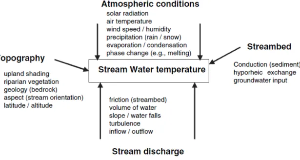
- Water temperature and abiotic factors
- Water Framework Directive
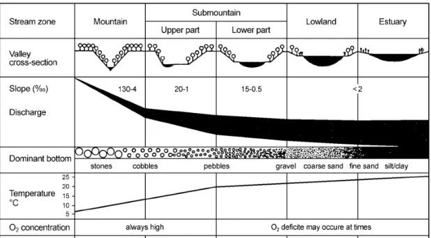
- Fish regions and Fish Zone Index
- Climate change and fish distribution
- Stream temperature modeling approaches
12 Introduction and problem definition water temperature reaches its minimum in the early morning and its maximum in the late afternoon (PRATS et al., 2010). Introduction and problem definition 17 parametric models are not so widely used because of their limited reliability (BENYAHYA et al., 2007).
Data and methods
- Data sources
- Abiotic data
- Biotic data
- Error elimination, data preparation and review
- Error elimination and data preparation
- Data review
- Abiotic factors of influence to stream temperature
- Correlation analysis
- Factor analysis
- Abiotic factors influenced by climate change
- Stream temperature model
- Data clustering
- Regression analysis
- Cross tabulation
- Validation
- Prediction of future stream temperature and fish assemblage
Through the location of HZB gauges in CCM2 (V2.1), the main basin of each area can be determined as well as the extent of the upstream basin. Finally, the developed stream temperature and fish assemblage models were used to predict future water temperatures and fish assemblages under the influence of climate change.
Results
Data review and selection: HZB gauges
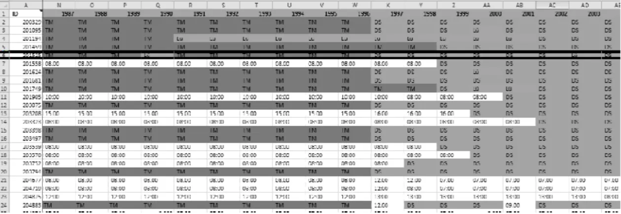
- Preliminary selection and measurement times
- Hydropower influence and river morphology
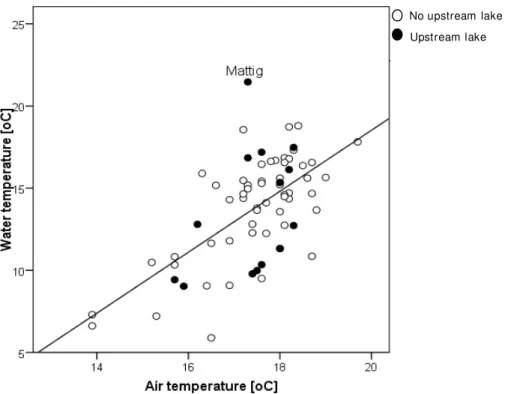
- Lake influence
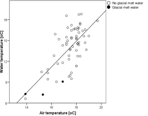
- Glacial influence
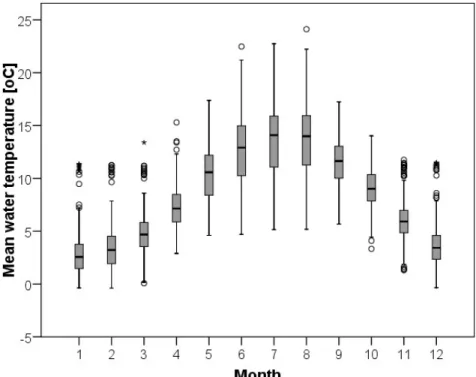
- Water temperature
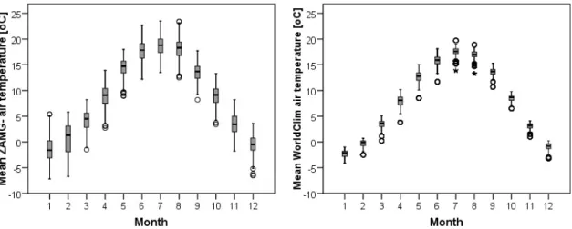
- Air temperature
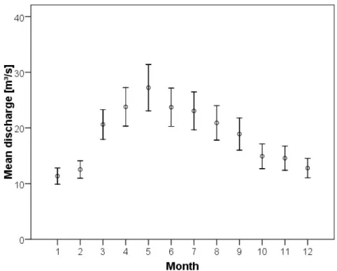
- Discharge
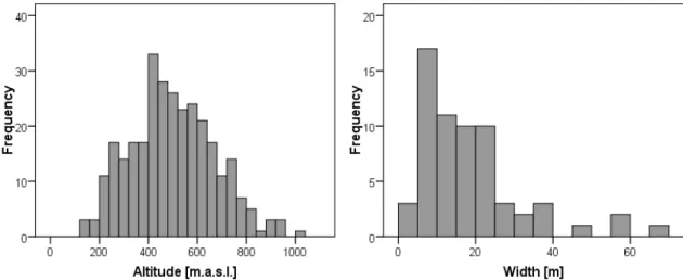
- River size and location of gauge
- Ecoregions
- Fish regions
- Stream order
- Summary
- Stream temperature Trends
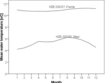
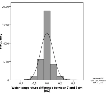
As Figure 3.4 shows, although they are in the lower part of the graph, none of the three rivers can be considered an outlier, and therefore they were not excluded from the dataset. As Figure 3-6 shows, the standard deviation is greatest in the summer and smallest in the winter months. As Figure 3-9 shows, the highest values are observed in May and the lowest in January.
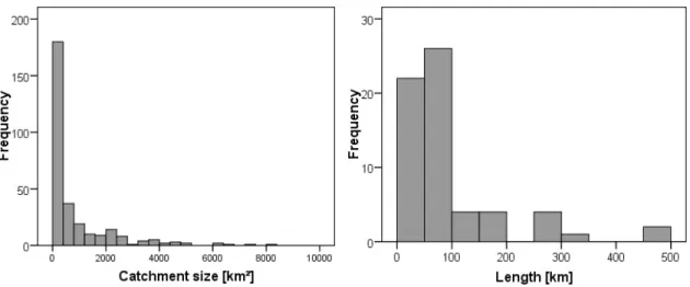
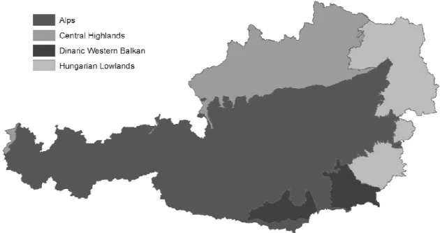
84% of the river sections in the relevant HZB locations have a catchment area below 500 km2, as shown in Figure 3.12. As Figure 3.17 shows, more than half of the stations are in the central highlands, 22 in the alpine.
Data review and selection: Fish sampling sites
- Site selection
- Geographic location
- Fish distribution
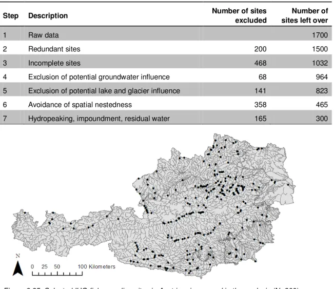
An overview of the reasons for the elimination of fish sampling sites can be seen in table 3.3. The distribution of the sampling sites in Austria is uneven, as several sites are located in the central and eastern part of Austria, as shown in Figure 3.25. The size of the catchment and the distance from the source as well as the altitude of the localities vary greatly.
The distance from the source varies between 5 and 298 km, with more than half of the sites located within 50 km of the source. Out of the 300 fish sampling sites, the majority are located in the trout region, as shown in Figure 3.30.
Abiotic factors significantly influencing water temperature
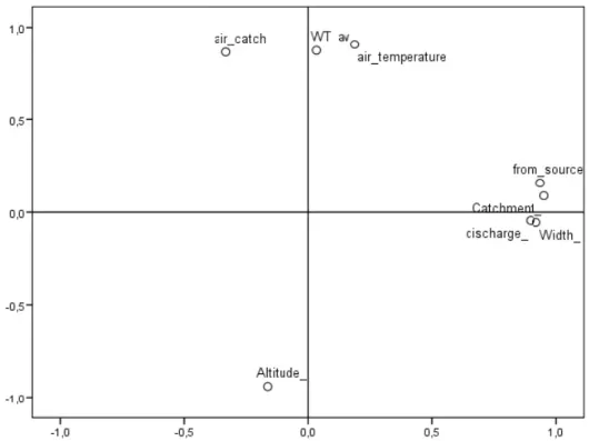
The factor graph (figure 3.34) shows the variables in the factor space, visualizing the relationship and loadings, where the axis represents the components. Just as the correlations differ when the data are divided into groups according to river width or catchment size, the factor plot differs strongly, as shown in figure 3.35, where the second catchment class (188-331 km2; corresponding to table 3.6) is taken as an example. It can be noted that the two groups are not as defined as in figure 3.34, and that the distance from the source is now in line with air and water temperature.
N=63) WT_av = Water temperature, from_source = distance from source and air catchment = average air temperature in the catchment. WT_av = Water temperature, from_source = distance from source and air catchment = average air temperature in the catchment.
Climate change and future scenarios
- Abiotic factors influenced by climate change
- Climate change scenarios
- Downscaling of climate change scenarios
- Future air temperature
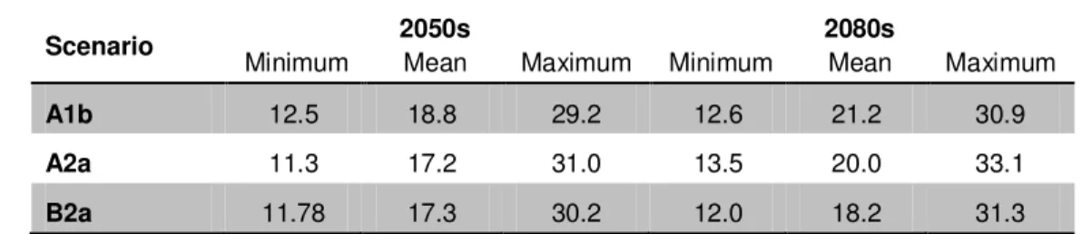
It is based on the sum of anomalies interpolated on the same high-resolution monthly climate surfaces from WorldClim (RAMIREZ-VILLEGAS & JARVIS, 2010), as used in this thesis, and is available for three emission scenarios (A1b, A2a and B2a). For this reason and the fact that the model is based on WorldClim data, which guarantees comparability, the statistically reduced data of the delta method were chosen. If the average temperature increase is compared to actual temperatures, as in Figures 3.37 and 3.38, it can be seen that the temperature increase is predicted to be greater in areas with lower temperatures.
It can also be noted that the temperature increase dependent on current air temperatures varies between the different scenarios, especially in the 2050s. While scenario A1b predicts a proportional increase, scenario B2a predicts a much stronger temperature increase for areas with relatively low temperatures.

Stream temperature model
- Regression model
- Crosstab model
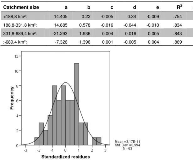
WT* = estimated morning water temperature at site s in month m (°C) ACs,m = average air temperature for site s' catchment in month m (°C) Cs = catchment size of site s (km²). In July, for example, the four variables catchment air temperature, catchment size, distance from the source and altitude explain the variability of the water temperature with an adjusted coefficient of determination of up to 0.83 and a significance level of 0.001. If the observed and predicted stream temperatures are plotted against the mean air temperature in each catchment, the lines of best fit differ by less than 0.3°C, as shown in figure 3.40.
Site 204925 in July 1997, for example, exhibits features summarized in mega-variable 212, which accumulates in profile variable classified 5 and therefore exhibits a flow temperature between 14 and 17°C. If, for example, the air temperature were to increase by 5°C in the future, the new profile variable would be 412 and the area would then be classified as profile variable classified 6, with the future stream temperature being estimated to be above 18°C.
Stream temperature and fish distribution
- Stream temperature- Fish Zone Index correlation
- Stream temperature- Salmonidae/Cyprinidae proportion
- Trout and Grayling distribution
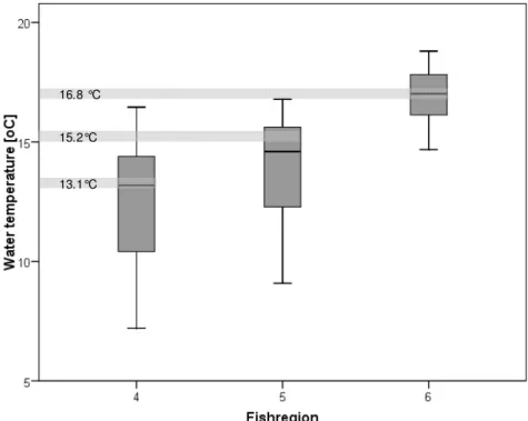
There is a strong correlation (ρ= 0.77) between the estimated stream temperature in July and the Fishing Zone Index, as shown in figure 3.44. The water temperature in the trout region (FizI~3.8) has the widest spread, with values from 7° to 15° Celsius. As can be seen, there is practically no difference in the temperature ranges between the two ways in which dominance was defined.
It can further be noted that 15°C is the temperature below and above which Salmonidae and Cyprinidae occur respectively, thus defining the boundary between Rhithral and Potamal in the data set. Similar to the flow temperature-FiZI ratio there is a correlation between water temperature and SCI, as shown in Figure 3.46.
Stream temperature and fish distribution under the influence of climate change
- Stream temperature
- Fish assemblage
The frequency distribution of potential fish zones should change along with FiZI. It can be observed that the share of areas in MR is expected to decrease drastically by 2080, especially according to scenarios A1b and A2a. All scenarios predict a large increase in sites in HR, making it the region with the highest frequency of fish sampling sites by 2080.
Although the number of locations in the EP is expected to increase, this increase is predicted to be relatively small compared to the larger number in the HR and MP. The vast majority of sites are expected to be allocated to the HR by 2050 and while this is still expected to be the most frequent fishing region in the 2080s, the gap to the number of sites in the Potamal has narrowed significantly.
Summary of results
Discussion
Dataset
- Water temperature data
- Air temperature
- Fish sampling sites
However, to ensure the applicability of the model across the country, an even distribution of the countries used for its development is required. Therefore, it cannot be guaranteed that the developed model is applicable to the whole of Austria, but it is valid for the central and eastern parts of the country. From these sites, 300 sites were selected with complete information and no human-induced changes in the water temperature regime.
82 However, discussion can be explained by the fact that most of the country's rivers are Rithral waters. As with the HZB tracks, the majority of the sites are in central Austria, with just under 4% in the west.
Abiotic factors influential on water temperature
One reason for this could be the increased occurrence of glaciers, lakes and reservoirs (SCHIMON et al., 2011) in the western part of the country, which constitute three of the criteria used for the exclusion of sites. However, the fact that the distribution of the fish sampling sites matches the distribution of the water temperature gauges supports the accuracy of the results, while bearing in mind the aforementioned limited applicability of the model in Western Austria.
Abiotic factors influenced by climate change and feasible predictions of such
SDMs are based on statistical relationships, rely on accurate baseline information (UNFCCC, 2011) and data are available for the whole world - especially Europe. One dataset based on SDMs provided by the CIAT relies on the same baseline temperature data used to develop the stream temperature models (WorldClim). This, and the fact that a limited number of RCMs are freely available, is the reason why this dataset was chosen as the source of future air temperatures.
To ensure compatibility between the different scenarios, data based on the HADCM3 was selected. This GCM has been used by the IPCC and has been assessed as an accurate model with its main deficiencies in tropical latitudes, as summarized by the German Climate Computing Center (Deutsches Klimarechenzentrum, DKRZ) (2003) and BARONTINI et al.
Stream temperature model
- Regression model
- Cross tabulation model
84 Discussion since the value for each month for each year was the same meant that stream temperature had to be averaged accordingly. These results can be said to be satisfactory since comparable studies achieved similar exploratory values (e.g. Furthermore, the model was developed only on the basis of one year, 2001, and the best coefficients of determination were found in August.
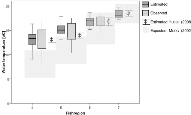
However, the mean values for MR and HR are estimated to be about 1°C lower than the values estimated in this thesis. For example, if the model were to be based on measurements along the length of a river, the exploration value is likely to increase and predictions of future stream temperature are likely to be possible.
Water temperatures and fish assemblages under the influence of climate change
- Current fish assemblage and water temperature
- Future stream temperature
- Future fish assemblage
Considering the figure below, the conclusion seems to be that most of the distribution of trout in the region is consistent with the literature (HUET, 1959; JOBLING, 1981; KÜTTEL et al., 2002). In particular, flow is expected to decrease by up to 25% in the Alpine region and increase by about 45% in the northeast of the country (STANZEL & NACHTNEBEL, 2010). Furthermore, the overall information obtained from this approach can be considered reasonable, as the results indicating a stronger shift towards Cyprinidae dominance are in line with the FiZI model outcome.
As visualized by SPINDLER (1997) in a table (Appendix I), none of the species occurs in only one fishing area. A reduction in salmonid distribution is also expected to have an effect on the aquatic food web, placing additional pressure on species in the upper fishing areas (MEILI et al., 2004).
Conclusion and outlook
Long-term changes within invertebrate and fish communities of the Upper Rhone River: effects of climatic factors. Geochemistry of the Rhine River and the upper Danube: Recent trends and lithological influence on baselines. Summary report: Contribution of Working Groups I, II and III to the Fourth Assessment Report of the Intergovernmental Panel on Climate Change.
Temporal variability in the thermal regime of the lower reaches of the River Ebro (Spain) and change due to anthropogenic factors. Potential habitat loss and population fragmentation for cold-water fish in the North Platte River drainage of the Rocky Mountains: response to climate change.
Asp (Aspius aspius) Kessler's Gudgeon, (Romanogobio kessleri) Zingel (Zingel zinge) Ide, Orfe (Leuciscus idus) Snoekbaars (Sander lucioperca) Schraetzer, gestreepte pos (Gymnocephalus schraetzer) Balon's pos. Gymnocephalus baloni) Zilverbrasem (Blicca bjoerkna). Zope (Cyprinus ballerus) Spined Loach (Cobitis taenia) Golden Spined Loach (Sabanejewia balcanica) Ziege, Sabelkarper (Pelecus knifetratus). Gymnocephalus cernuus) Meerval (Silurus glanis) Zeelt, doktersvis (Tinca tinca).
109