Globalization and the Gains from Variety The Case of a Small Open Economy
Lukas Mohler
University of Basel
Vienna, December 12, 2008
Introduction Motivation
Introduction
– We observe a high growth in imported variety. Example: Broda and Weinstein (2006) report an increase of imported variety of 67% for the U.S. from 1972 to 2001.
– What are the welfare gains from this increased imported product variety? There are many case studies and calibrated models (Romer (1994), Klenow and Rodriguez-Clare (1997)) that try to answer that question. – Broda and Weinstein (2006) are the first who structurally estimate these
gains: 2.6% of GDP in the U.S. between 1972 and 2001.
Introduction Motivation
Introduction
– We observe a high growth in imported variety. Example: Broda and Weinstein (2006) report an increase of imported variety of 67% for the U.S. from 1972 to 2001.
– What are the welfare gains from this increased imported product variety?
There are many case studies and calibrated models (Romer (1994), Klenow and Rodriguez-Clare (1997)) that try to answer that question.
– Broda and Weinstein (2006) are the first who structurally estimate these gains: 2.6% of GDP in the U.S. between 1972 and 2001.
Introduction Literature
Literature
– Feenstra (AER 1994)
• Set up a CES-model where new varieties lower unit-costs.
• Derived a corrected price index that accounts for variety change.
• Developed a stochastic model to estimate the elasticities of substitution.
• Showed that conventional import price indices are biased upwards.
– Broda and Weinstein (QJE 2006)
• Apply this to many imported product categories using disaggregated trade data.
• Aggregating, they find a welfare gain of 2.6% of the GDP in the US between 1972 and 2001.
Introduction Contributions
Contributions
– Estimating the gains from imported variety for Switzerland and the U.S.
for the period of 1990 to 2006.
– Analyzing these gains with special attention to the particularities of a Small Open Economy (SOE).
– Proposing an alternative definition of traded variety and presenting the results for this new specification.
Methodology Overview
Methodology: Overview
– The calculation of the gains from variety can be divided into 3 steps:
• Estimate the elasticity of substitution for each product category.
• Calculate the corrected import price index and the aggregate bias.
• Compute gains from variety by allowing for the domestic economy.
Methodology Corrected Import Price Index
The Corrected Price Index
– The Feenstra Price Indexπg for goodg including varietiesc:
πg =Pg(Ig)
„ λgt
λgt−1
«1/(σg−1)
, where (1)
λgt= P
c∈Igpgctxgct
P
c∈Igtpgctxgct
,
λgt−1= P
c∈Igpgct−1xgct−1
P
c∈Igt−1pgct−1xgct−1
.
Ig is called the common set.
Methodology Corrected Import Price Index
The Corrected Price Index
– The Feenstra Price Indexπg for goodg including varietiesc:
πg =Pg(Ig)
„ λgt
λgt−1
«1/(σg−1)
, where (1)
λgt= P
c∈Igpgctxgct
P
c∈Igtpgctxgct
,
λgt−1= P
c∈Igpgct−1xgct−1
P
c∈Igt−1pgct−1xgct−1
.
Ig is called the common set.
Methodology Corrected Import Price Index
The Corrected Price Index
– The Feenstra Price Indexπg for goodg including varietiesc:
πg =Pg(Ig)
„ λgt
λgt−1
«1/(σg−1)
, where (1)
λgt= P
c∈Igpgctxgct
P
c∈Igtpgctxgct
,
λgt−1= P
c∈Igpgct−1xgct−1
P
c∈Igt−1pgct−1xgct−1
.
Ig is called the common set.
Methodology Corrected Import Price Index
The Corrected Price Index
– The Feenstra Price Indexπg for goodg including varietiesc:
πg =Pg(Ig)
„ λgt
λgt−1
«1/(σg−1)
, where (1)
λgt= P
c∈Igpgctxgct
P
c∈Igtpgctxgct
,
λgt−1= P
c∈Igpgct−1xgct−1
P
c∈Igt−1pgct−1xgct−1
.
Ig is called the common set.
Methodology Computing the Gains from Variety
Computing the Gains from Variety
– Aggregating all theπg’s we get the aggregated import price index Π and thus the aggregate bias in the conventional import price index.
– Since no information about the domestic structure of the economy is known, a simple Krugman-like economy is assumed.
Results The Gains from Variety
Results: The Gains from Variety
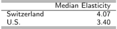
– Imported variety increases by 23’112 varieties in Switzerland and by 39’143 varieties in the U.S. Relative: 34% and 43%.
– The estimation of the elasticities of substitution yields the following result: Table 1: Median Elasticities
Median Elasticity
Switzerland 4.07
U.S. 3.40
– Table 2 shows the estimated gains from variety for Switzerland and the U.S.
Table 2: Gains from Imported Variety, Switzerland and U.S. 1990-2006
Agg. Bias GFV Switzerland 3.85% 1.86%
U.S. 14.23% 1.55%
Results The Gains from Variety
Results: The Gains from Variety
– Imported variety increases by 23’112 varieties in Switzerland and by 39’143 varieties in the U.S. Relative: 34% and 43%.
– The estimation of the elasticities of substitution yields the following result:
Table 1: Median Elasticities Median Elasticity
Switzerland 4.07
U.S. 3.40
– Table 2 shows the estimated gains from variety for Switzerland and the U.S.
Table 2: Gains from Imported Variety, Switzerland and U.S. 1990-2006
Agg. Bias GFV Switzerland 3.85% 1.86%
U.S. 14.23% 1.55%
Results Analyzing the Gains from Variety
Analyzing the Gains from Variety I
– Within this framework, the gains from variety can differ between countries due to mainly 3 reasons:
• Differences between the import shares.
• A different number of new varieties imported at high values.
• Differences in the degree of differentiation of the imported varieties. Agg. Bias GFV
Switzerland 3.85% 1.86%
U.S. 14.23% 1.55%
Results Analyzing the Gains from Variety
Analyzing the Gains from Variety I
– Within this framework, the gains from variety can differ between countries due to mainly 3 reasons:
• Differences between the import shares.
• A different number of new varieties imported at high values.
• Differences in the degree of differentiation of the imported varieties.
Agg. Bias GFV Switzerland 3.85% 1.86%
U.S. 14.23% 1.55%
Results Analyzing the Gains from Variety
Analyzing the Gains from Variety I
– Within this framework, the gains from variety can differ between countries due to mainly 3 reasons:
• Differences between the import shares.
• A different number of new varieties imported at high values.
• Differences in the degree of differentiation of the imported varieties.
Agg. Bias GFV Switzerland 3.85% 1.86%
U.S. 14.23% 1.55%
Results Analyzing the Gains from Variety
Analyzing the Gains from Variety II
– Table 3 shows the relative differences the aggregate import price index of Switzerland relative to the US.
Table 3: Relative Differences of the Aggregate Bias Under Fixed Elasticities
variable σ= 2 σ= 4 σ= 8 σ= 15 Rel. difference in bias -72.9% -62.9% -65.5% -66.2% -66.5%
– As a conclusion, the majority of the difference in the aggregate bias, namely about 90%, is due to the lower variety growth in Switzerland. The rest of the difference is due to the higher elasticities of substitution for Swiss import goods.
Proposing a Definition of Traded Varieties Some Problems
Some Problems
– The results shown above heavily depend on the definition of a variety:
• Different data set, different definition.
• Number of “actual” varieties.
– In search of a general definition for traded varieties, I propose a slightly changed version of Feenstra’s lambda ratios. I want to illustrate that
• another definition of a traded variety changes the GFV radically.
• the lambda ratios are a first step towards a more general definition of traded varieties.
Proposing a Definition of Traded Varieties
Proposing a Definition of Traded Varieties I
Proposition:
The lambda ratio is defined as
λgt
λgt−1
=
P
c∈Igpgctxgct P
c∈Igtpgctxgct P
c∈Igpgct−1xgct−1 P
c∈Igt−1pgct−1xgct−1
To obtain a new version of the price index bias, the setIg contains but one artificial variety with constant expenditure. Thus, the lambda ratio simplifies to
λgt
λgt−1
= P
c∈Igt−1pgct−1xgct−1
P
c∈Igtpgctxgct
.
Proposing a Definition of Traded Varieties Critical Assessment
Critical Assessment
– This “new” definition of the lambda ratios has the following advantages and disadvantages:
λgt
λgt−1
= P
c∈Igt−1pgct−1xgct−1
P
c∈Igtpgctxgct
.
• - Higher expenditure on a specific product leads directly to a higher variety.
• + But only if the elasticities of substitution is low, this also lower the import price index.
• + Independent of the data set used.
Proposing a Definition of Traded Varieties Results
Results
– Table 4 presents the gains from variety for Switzerland and the U.S. using the new specification:
Original New
Agg. Bias GFV Agg. Bias GFV Switzerland 3.85% 1.86% 14.67% 7.74%
U.S. 14.23% 1.55% 34.79% 4.37%
Proposing a Definition of Traded Varieties Results
Results
– Table 4 presents the gains from variety for Switzerland and the U.S. using the new specification:
Original New
Agg. Bias GFV Agg. Bias GFV Switzerland 3.85% 1.86% 14.67% 7.74%
U.S. 14.23% 1.55% 34.79% 4.37%
Conclusions
Conclusions
– I calculate the gains from variety in Switzerland and the U.S. for the period of 1990 to 2006. Despite the differences between these countries, the estimates of the gains from variety are close, namely 1.9% and 1.6%.
– Comparing a SOE like Switzerland with the U.S., the aggregate import bias is always larger in the large economy. This is mostly due to the higher increase in imported variety and to a lesser extent to the lower elasticities of substitution. Due to the larger import share, the gains from variety in a SOE may still be higher. I also argue that this may be true for other OECD countries.
– I propose a different and more general definition of traded variety, slightly changing Feenstra’s lambda ratios. I show that the differences in the gains from variety can be substantial using another specification.
Conclusions
Conclusions
– I calculate the gains from variety in Switzerland and the U.S. for the period of 1990 to 2006. Despite the differences between these countries, the estimates of the gains from variety are close, namely 1.9% and 1.6%.
– Comparing a SOE like Switzerland with the U.S., the aggregate import bias is always larger in the large economy. This is mostly due to the higher increase in imported variety and to a lesser extent to the lower elasticities of substitution. Due to the larger import share, the gains from variety in a SOE may still be higher. I also argue that this may be true for other OECD countries.
– I propose a different and more general definition of traded variety, slightly changing Feenstra’s lambda ratios. I show that the differences in the gains from variety can be substantial using another specification.