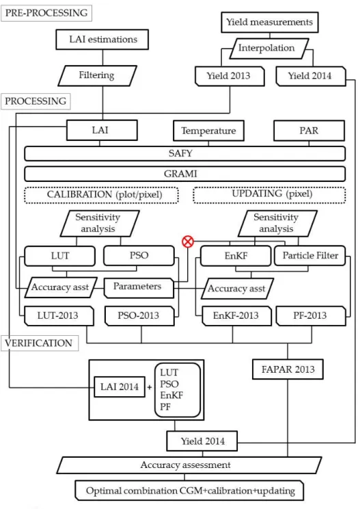
The calibration of the SAFY model at plot scale using PSO and the updating at pixel scale using PF yielded a suitable average accuracy at both regional (2.5%) and plot scale (10.5%). I would like to thank the researchers of the Institute for Surveying, Remote Sensing and Land Information (IVFL).
Introduction
Objetives of the research
The global research goal is to develop an assimilation method based on a simple crop growth model to estimate maize yield in the Marchfeld region with a minimum input data requirement.
Retrieval of vegetation bio-physical variables using EO data
- Introduction
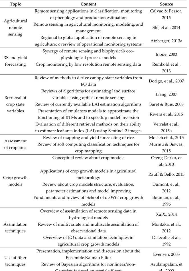
- Quantitative analysis of Research
- General classification of bio-physical retrieval techniques
- Empirical methods
- Mono-variate approaches
- Multi-variate approaches
- Drawbacks of empirical approaches
- Semi-empirical methods
- Predictive equations
- Simplified canopy reflectance models based on Beer’s law
- Physical methods
- General conditions affecting RTM performance
- Examples of RTM’s used in agricultural remote sensing
- Model inversion algorithms
- Model inversion and ill-posedness
- Coping with the ill-posedness of the model inversion
- Pros and cons of different inversion methods
- Overview of retrieval of vegetation bio-physical variables using EO data
Vuolo et al., (2013) applied a similar semi-empirical model to derive time series of LAI maps using an exponential relationship between LAI and the Weighted Difference Vegetation Index (Clevers, 1989) and reported a good performance. Vuolo, et al (2010) compared the suitability of empirical and RTM approaches to estimate LAI, leaf green chlorophyll content (CCC) and leaf chlorophyll content (LCC) using RapidEye data.
Assimilating remotely retrieved biophysical variables in crop models
Introduction
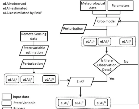
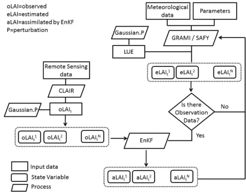
In Section 3.3, we briefly introduce the three main techniques for assimilating remotely sensed biophysical variables into crop models: forcing, calibration, and updating. Finally, in Section 3.9 we present an overview of crop growth modeling and monitoring by combining CGMs and EO data.
Crop biomass and yield estimation
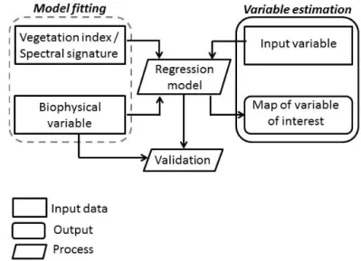
- Empirical models
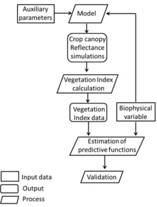
- Semi-empirical models
- Crop simulation models
- Complex crop simulation models
By combining remote sensing and crop modeling, the synergy between the two techniques is exploited (Delécolle et al., 1992). However, such strategies come at the cost of reducing the predictive capacity of the model (Wallach et al., 2002).
Main approaches for assimilating EO data in crop growth models
A way to identify simplification strategies is to use tools such as PYGMALEO (Cournède et al. Unlike calibration, updating allows to model state variables directly, without requiring all remote sensing observations to be considered.
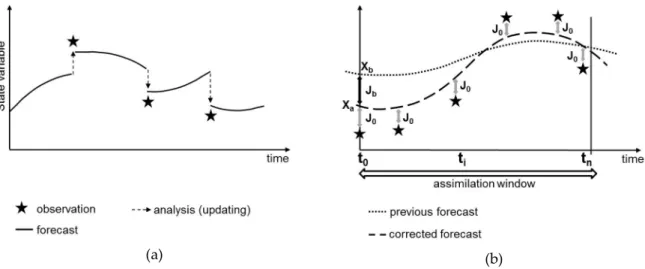
Forcing
After calibration, the model is run again to produce a new set of simulated values (Figure 7b). Because it is computationally simple, a major drawback of the forcing strategy is that the model accuracy is strongly determined by the accuracy and number of remote sensing observations.
Calibration: re-initialization and re-parameterization
- Sensitivity analysis
- Remote sensing data availability
- Errors in the EO-retrieved state variables
- Effect of fixed parameters and number of parameters to be calibrated
- Compensation between parameters and ill-posedness of the calibration
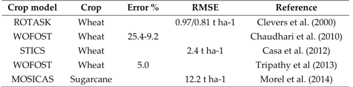
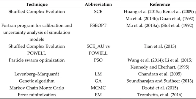
Therefore, other assimilation strategies seem more appropriate than the forcing method (Delécolle, 1992; Li et al., 2011). Other factors also strongly influence the calibration performance under adverse conditions, such as (1) the complexity of the model, (2) the criterion used to calculate the calibration error, (3) the algorithm used to meet the optimal parameters to meet. values (Table 6), and (4) the criteria used to compare different algorithms (Wallach, et al. 2001).
Updating
- Linear Kalman filter (LKf)
- Extended Kalman filter (EKF)
- Ensemble Kalman filter (EnKF)
- Ensemble square root filter (EnSRF)
- Particle Filter (PF)
- Versatility of updating techniques
- Important aspects for implementing ensemble updating filters
- Ensemble size
- Time step
- Normality of the residuals
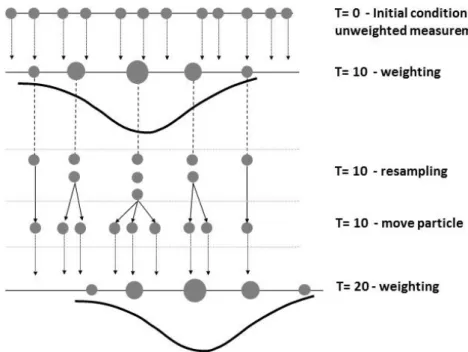
The error for each particle relative to the center of the observation distribution (the mean) is calculated. The choice of ensemble size requires a compromise between the computational cost and the accuracy of the covariance matrices (Trudinger, et al. 2008).
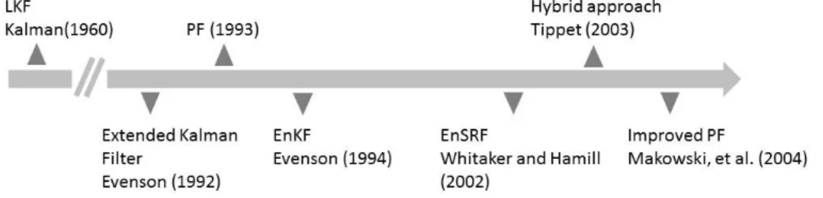
Hybrid approaches
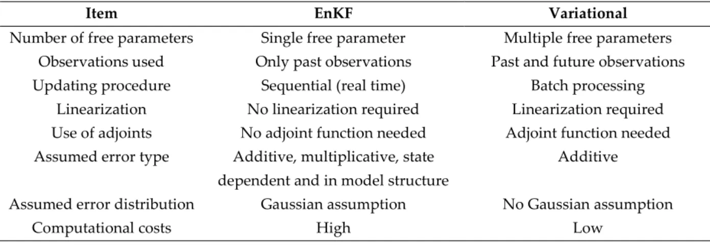
The size of the assimilation step is another factor that influences the stability of the assimilated profile. The use of the adjunct or tangent linear model is avoided, increasing assimilation precision and reducing computational costs related to EnKF (Tian, et al., 2008).
Aspects related to the assimilated EO data
- Spatial resolution
- Temporal resolution and timing of observations
- Combining data from several sensors
- Assimilation of reflectances instead of bio-physical variables
- Identification and modeling of key phenological events
- Developments in geophysics
Simultaneous assimilation of remotely sensed data from different sensors (optical and radar) into a crop model is feasible and reduces the effect of cloud cover (Prèvot, et al. 2003). The performance of the EnKF was even worse compared to the crop model run with default parameters. Unfortunately, RS contributes very little to the observation of plant phenological phases (Delecolle et al., 1992).
Overview of the assimilation of retrieved EO data in CGMs
Therefore, phenological events must be estimated with high accuracy to achieve a realistic crop growth simulation (Moulin et al., 1995). A number of factors related to the quality of the EO data affect the accuracy of data assimilation in crop models. The fusion of remote sensing observations from different sensors is an alternative to minimize spatial and temporal data limitations (Prèvot, et al. 2003).
Materials
- Study area
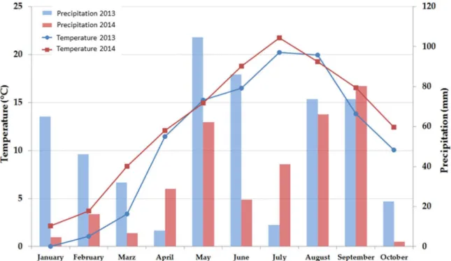
- Meteorological data
- Satellite Data
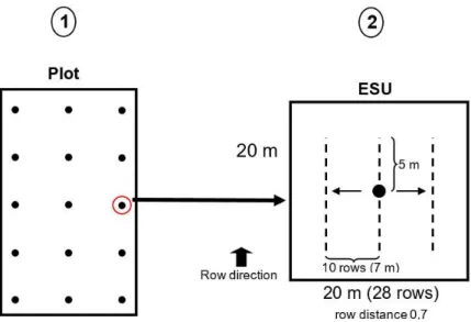
- Field measurements
- Leaf Area Index measurements
- Yield crop estimation in field
Estimates of LAI by LICOR 2200 are primarily affected by two types of errors; underestimation due to the non-random placement of canopy elements and overestimation due to the incapacity. The effect of non-random placement of crown elements is maximized at the beginning of plant growth, especially for crops such as maize with a relatively large row space. In each sample, the number of ears was counted and two ears were selected to estimate the number of kernels per ear. ear as well as the weight of the core.
Method
GRAMI and SAFY crop simulation models
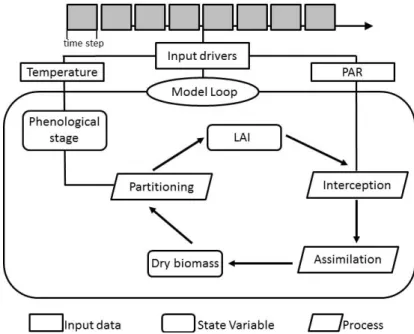
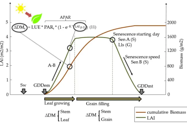
The models run from the date of sowing to the day of full leaf senescence and consider three cardinal stages of growth: urgency, flowering and maturity. The leaf elongation period starts from emergence to flowering and the grain filling period from flowering to maturity. Before flowering, the formation of new leaf tissue stops and photoassimils are directed to grain growth.
LAI estimation
The model design considers that cereals have an initial period in which most of the aboveground dry mass consists of leaf tissue. Therefore, it could be an indicator of the success of agricultural practices such as irrigation and fertilization. The ratio ρs nir/ρs red is called the slope of the soil line, a linear ratio of the red and near-infrared reflectance of bare soil that represents the effects of the soil background on the calculation of the vegetation index.
Sensitivity analysis
- Generating a reference simulation
- Univariate sensitivity analysis
- Parameter correlation analysis
- Sensitivity analysis of LUT and PSO to LAI data
WDVI = ρnir – (ρred * ρs nir/ρmiddle) (6) where ρred and ρnir represent the reflectance in the red and near-infrared channels, respectively. The robustness of the LUT and PSO approaches for accurate calibration of the GRAMI and SAFY models was tested using synthetic LAI data. The objective of the sensitivity analysis was to simulate the effect of an error in the EO data, such as the presence of clouds, atmospheric noise, or inaccuracy of the inversion algorithm to obtain LAI in CGM calibration.
Filtering of Leaf Area Index estimations
The sensitivity was assessed by comparing the reference yield and phenology with the estimates obtained by SAFY and GRAMI calibrated by LUT and PSO. A set of synthetic LAI observations was generated using the reference LAI data series and adding noise to the reference curve by the Monte Carlo approach. The Whittaker filter was chosen because it is easy to implement, it is capable of processing large amounts of data, and it is controlled by a unique parameter (λ) that can be calibrated visually or by a cross-validation approach (Atzberger and Eilers, 2011). ).
Calibration of CGM parameters
- Iterative Look up Table (iLUT)
- Particle Swarm Optimization algorithm
Biomass was calculated as the average of simulations obtained with selected LUT records. Finally, vit+1 and xit+1 are the velocity and position of particle i at time t+1 (Kim et al, 2013). In addition, the number of parameters to be optimized was tested to evaluate the effect of ill-posed problems in the PSO algorithm.
LAI updating approach
- Ensemble Kalman filter
- Particle Filter
The GRAMI and SAFY models used in the iLUT and PSO sensitivity analysis were implemented. Variables and value range tested in the sensitivity analysis of EnKF Observation and Model ensemble size from 50 to 500 particles. The values used in the sensitivity analysis were the same as in the EnKF.
Validation of GRAMI and SAFY models
Verification
General considerations
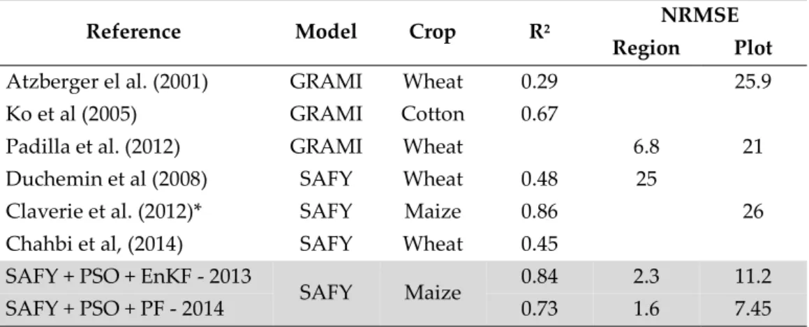
In the first part, the results of calibration and updating of GRAMI and SAFY models regarding yield observations for the 2013 season are presented and discussed (§ 5.1 to § 5.8). Then, in Section 5.9, we introduce the results of the verification of the techniques using yield observations of the 2014 season. Finally, we present an overview discussion of the most relevant points of our experiment and a comparison of the results obtained for both seasons with findings from similar previous research (§ 5.10).
Yield estimation by field sampling
LAI estimation using EO data
Sensitivity analyses of crop growth modelss
- Univariate sensitivity analysis
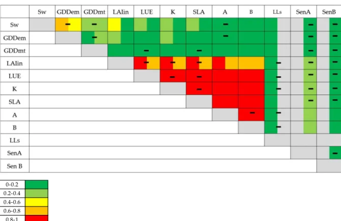
- Parameter correlation analysis
In SAFY, daily senescence of the leaf is calculated as a percentage of the biomass synthesized the day before the current loop. These last two parameters are related to the slope and the maximum value of the LAI curve (Figure 18). The diagram provides a good overview of the complexity of parameter calibration using LAI data series.
Yield estimation using calibrated GRAMI and SAFY models by the iterative LUT technique
- First step of iterative LUT calibration
- Cost function
- Criteria to extract LUT records
- LAI filtering
- Iterative LUT approach at plot scale
- LUT approach at pixel scale
The scatterplots between yield simulated and observed for the first and best iteration of the LUT for GRAMI (a, b) and SAFY (d, e) are outlined in Figure 28. Table 17 details the fixed and free parameters for the first and second steps of GRAMI and SAFY calibration at pixel scale. Fixed and free parameters in the first and second steps of GRAMI and SAFY calibration at pixel scale.

Yield estimation using calibrated GRAMI and SAFY models by the Particle Swarm
- PSO parameters sensitivity
- Optimum PSO parameter value
- Number of PSO repetitions
- Number of optimized parameters
- Cost function
- Application of PSO at plot and pixel scale
This increase is due to the inclusion of phenological parameters such as Sw, GDDem, GDDmt in the optimization routine. For both models, a significant reduction in yield estimation variability is observed in most plots (black bars). This can be explained by the fact that LAIin, SLA and K are included in the calibration.
Comparison between calibration approaches regarding yield crop estimation
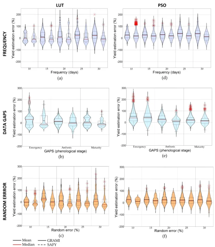
- Sensitivity analysis of LUT and PSO to LAI data
- Crop yield estimation
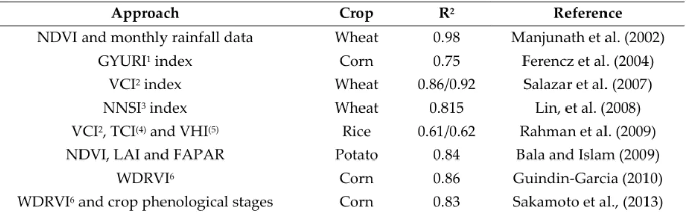
- Crop yield forecasting
Finally, Fig. 32(c) and (f) show the sensitivity of LUT and PSO to random errors in the LAI data. The effect of the random error in the estimation of GDD on anthesis is similar for both calibration techniques. In addition, the mean of the error tends to overestimate the GDD to anthesis, as was observed in Fig. 33(c).
Yield estimations using updated GRAMI and SAFY models
- Parameter sensitivity
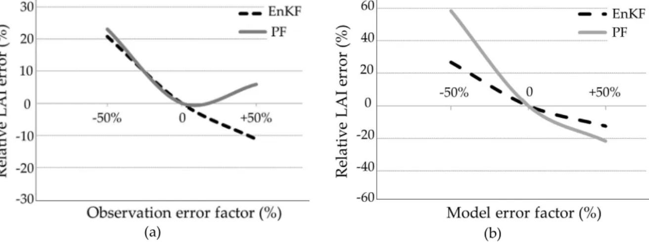
The effect of underestimating the observation error is similar for EnKF and PF, with an error increase of 20. The impact is stronger for PF with a reduction in LAI update accuracy of about 60%. Together, this demonstrates the strong influence of CGM on the accuracy of yield estimation, regardless of the calibration technique.
Validation of GRAMI and SAFY parameters
The scatterplots of the combination SAFY + PSO + EnKF and SAFY calibrated at pixel scale by PSO with three free parameters are compared in Figure 37. The effect of the source of phenological data and LUE on the yield error estimate at plot scale (EEP) by Monteith -comparison is depicted in Figure 38. Effect of the phenology extraction method and LUE on the yield estimation error at plot scale (EEP) using Monteith equation.
Verification
However, it is worth mentioning that most of the maize fields in the study area are irrigated. For example, for the GRAMI model, the best iLUT performance was obtained using the first iteration instead of the best iteration as in season 2013. In addition, the graph shows a greater variation of the yield estimates with respect to 2013; the average CV was increased by 22%.
Discussion
- Reference data of maize yield
- LAI observations
- Reference GRAMI and SAFY parameter values
- Sensitivity of biomass and LAI to parameters variation
- Calibration of GRAMI and SAFY parameters
- Updating of LAI in GRAMI and SAFY models
- Model performance for simulating crop yield
Then, the error in the yield estimation was reduced due to the new selected parameter levels. We recommend assessing the effect of the parameters' dispersion in the accuracy of the CGM considering the calibration of multi (inter-) correlated parameters (unfortunate problem). A lower variability of the yield estimation was achieved by calibrating the CGM parameters using PSO.
Conclusions and recommendations
- General overview about crop monitoring
- Retrieval of vegetation bio-physical variables
- Assimilating remotely retrieved biophysical variables in crop models
- Maize yield estimation by using GRAMI and SAFY models
- Sensitivity analyze of GRAMI and SAFY parameters
- Sensitivity of LUT and PSO to the error level, frequency and gaps of LAI data
- Yield estimation using calibrated GRAMI and SAFY models by iLUT and PSO techniques
- Updating of GRAMI and SAFY models using EnKF and PF
- Recommendations and further research
The parameters with a stronger influence in LAI calibration are SLA, A, B and LUE for both models. The present work demonstrates an increase in yield estimation accuracy using pixels. Given the good performance of PF in the 2013 and 2014 seasons, we recommend plot-scale SAFY model calibration using PSO and pixel-scale updates using PF.
Calibration of the SUCROS emergence and early growth module for sugar beet using optical remote sensing data assimilation. Improvement of winter wheat yield estimation by assimilation of the leaf area index from Landsat TM and MODIS data in the WOFOST model. Assimilation of Remote Sensing and Crop Model for LAI Estimation Based on Ensemble Kalman Filter.
Comparative evaluation of radiative transfer model inversion approaches for estimation of crop biophysical parameters. Using remote sensing data to estimate US winter wheat yield.
Index of tables
Index of figures
Index of abbreviations
CPF Convolutional particle filtering EEP Estimation error at scale plot EER Estimation error at regional scale EKF Extended Kalman filter.
Appendices
The curvature of the SPF function is controlled by the parameters A (defining the maximum value of the SPF curve) and B (defining the slope of the SPF curve). The grain biomass is calculated from the distribution yield coefficient (Py), which represents a percentage of the total biomass distributed on the grain each day during the period from flowering to maturity, instead of GRAMI, which is considered as a percentage (YPF) of daily produced biomass. The stepwise technique makes it possible to analyze the marginal effect of the inclusion of a new independent variable in the model.