Since it seems unlikely that the appropriate changes can occur in the short term, we think that the effects of the REP can also be verified by the implementation of future tax cuts (currently under consideration to mitigate the initial recession of 2008). .3. The remaining structure of the model contains firms that produce varieties in a monopolistically competitive manner. For simplicity, we assume that the 'segment' of varieties is equal to the population percentages of both countries.
1 2Esis is defined as the price of a unit of foreign currency in terms of local currency.
Producers and importers
Aggregation of consumers As we indicated in the previous section, economics includes both kinds of consumers: optimizers and rules of thumb. Note that we assume that each firm decides how much labor to hire (considering wages, see section 4.3) and distributes labor demand evenly among households (the type does not indicate any difference in marginal labor productivity). To analyze the producer maximization problem, we note that the law of large numbers can be applied because the number of firms is large, so we drop the highest indices of the Calvo price parameter.
Λjt marginal utility of nominal wealth of household j, Pm,t(i) is the corresponding vector of corresponding prices of domestically produced goods in the sector and T Cm,t+a(i)(·) is the (nominal) total cost of production in period t+a of the firm i domestic type m, which is a function of the total output of firm i in period t. Furthermore, ιm is the unity vector consisting of the corresponding number of ones equal to the number of markets, and (ϕm)a is the vector of Calvo probabilities for the price vector Pm,t(i) that remains unchanged for producer i of home type m. 2 4Please note that prices quoted by consumer importers are invoiced in domestic currency and exporters are invoiced in foreign currency.
It can be shown that three different Phillip curves can be derived if equation (34) is rewritten in terms of appropriate inflation rates.27.
Staggered wage setting
Equilibrium conditions
Fiscal policy
In this section we comment on the assumed fiscal and monetary policy followed by the home country.
Monetary policy
It is worth considering the marginal values of φ1, which means that the budget expansion is fully financed by: (a) taxes ifφ2= 1 or (b) deficit spending, ifφ2= 0. The intuition for the value of the previous feedback parameter is that BK it must raise the interest rate by more than any increase in inflation to raise the real interest rate, cool the economy, and return inflation to its target. McCallum, 1997] argues that policymakers' response is more accurate if it is based on lags rather than actual values of output and inflation.
In contrast, [Claridaet al., 2000], among others, argue that the rules in which the CB reacts to remote variables are optimal in the case of a quadratic objective function of the monetary authorities, which will also be used in this document. . The difference between backward-looking, contemporaneous and forward-looking monetary rules is mainly related to the information set of monetary policy makers. For example, in the case of a simultaneous rule, the target is the current inflation rate, on which the CB is assumed to have adequate information.
An interesting alternative to the rules above is one that chooses policy response values that minimize the present value of the SL's loss function (a weighted linear combination of deviations from the target variables and the instrument).
Shocks driving the economy
A rational expectation (RE) equilibrium is then a series of processes of the endogenous variables satisfying both first-order conditions (of corresponding optimal problems) and equilibrium conditions on all datas≥0 given the exogenous processes included in the vectorξt+s . The function Fθ:Λ3×R8−→Λis real inC2 parameterized by the real vectorθ∈Θ⊆Rp, where the dimension of the parameter space containing deep parameters is . Repeated replacement of equation (49) with (48) yields a system where yandv are sometimes included in the information set.
Model (48) has a solution at a fixed point known as the deterministic (Es[vs] =0) steady state. The steady state is a key element for the solution of our model given the fact that we use local approximation methods. It is primarily based on the systematic perturbation of the policy function around a steady state.
Third, the generalized eigenvalues of B1 and B2 are reorganized into Λ and Ω, in ascending order from left to right (Q0 and Z0 are reorganized accordingly). We will replicate the result of the positive multiplier of consumption for an expansionary fiscal policy, illustrated in Table 1. Keeping in mind that the parameterization is very important in the numerical simulation experiment, we first describe the chosen parameters before describing the effects of shocks. analyze. , 2 and 4, mentioned in the previous paragraph.
Calibration
Note that equation (52) is nothing more than an ANSWER, which allows us to calculate IRFs as well as variance decompositions conditional on the proposed calibration. With our parameterized model, policy makers can find out how interventions in different regimes (scenarios) will affect expected paths of sensible variables within an arbitrary probability confidence interval. The willingness to postpone consumption or the discount factor, β, is set to 0.99 according to a long-term (annual) nominal interest rate of 4%.
Since the observed price and wage stability depends on the Calvo parameter (see Sections 4.2 and 4.3), we assume that on average all wages and prices are revised once a year, so ϕH =ϕXH =ϕM F =ϕW = 0.75. With regard to the elasticity of the substitution of domestic and foreign goods, we assume that ηc= 1.8; and the degree of home bias is assumed to be ϕ= 0.5. For the AR(1) processes, we assume the following persistence parameters: (i) productivity, ρA, equal to 0.95; and (ii) government expenditure,ρg, equal to 0.85.
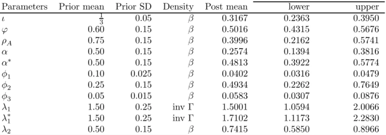
Therefore, the reaction parameter for inflation, λ1, is set equal to 1.5, without inertia, i.e. λ0 = 0, the corresponding output gap response parameter, λ2, is set equal to 0.5. The smoothing parameter, λ3, is assumed to be 0.8, which is consistent with a monetary policy having full effect after 5 quarters.
Numerical simulations
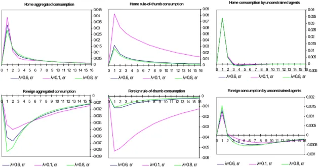
In Figure 2, we report a negative and purely temporary shock in money demand and its impact on consumption (resulting from an exogenous leftward shift in money demand). The immediate effect occurs on the money market when the nominal interest rate falls (in the first round the central bank does not react). Given the tradability of goods, foreign consumers without constraints anticipate a temporary opportunity to consume more due to the expansionary effect of foreign production resulting from higher exports to the home country.
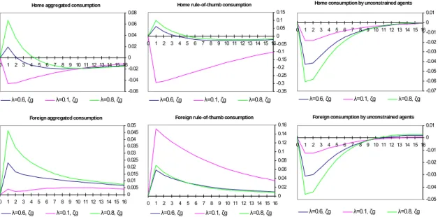
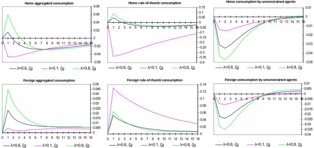
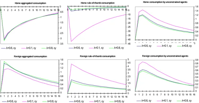
However, foreign consumers are less responsive to the impact due to the fall in disposable income due to higher foreign taxes to cover the issue of bonds to cover the trade deficit. In our view, the most interesting case to analyze relates to expansionary fiscal policies at home, as illustrated by the IRFs of Figures 3 and 4. This behavior is the result of the relatively large weight of 'rules of thumb' consumers in the economy which reverse the negative adjustment in consumption (according to the REP) in response to future government obligations.
For parameterisation where λr<0.45, the response of total consumption in the home economy remains negative within four years. Therefore, the crucial question that arises is which estimate of λr is supported by the US data. In addition, in the next subsection, we estimate the deep parameters of the model using Bayesian techniques.
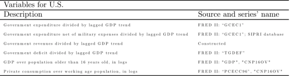
Data
Data into the DSGE model and the likelihood function
The former density is given directly by the measurement equation (53), while ys |Yso−1 is calculated by the Kalman filter.
Bayesian estimation: the likelihood meets prior densities
The idea behind Bayes' principle is to find a vector of parameters that maximizes the posterior density, given the prior and the likelihood based on the data. Θp(ˆyo|θ)p(θ)dθ is the unconditional data density, which, since it does not depend on the parameter vector being estimated, can be treated as a proportionality factor and accordingly can be neglected in the estimation process. The last term can be directly calculated from the given prior distributions of the estimated parameters.
To calculate the log-likelihood of the data, the Kalman filter is applied to the DSGE model solution (state-state representation) for the number of periods, T, provided by datayˆo. More accurate results for our sample can be derived via simulation given its non-standard form, using an approximation method around the optimum that generates a (large) sample of features using the Markov-Chain Monte Carlo (MCMC) algorithm. This is useful for characterizing the shape of the posterior distribution from which to draw inferences.
The Metropolis-Hastings algorithm is implemented using a jumping distribution to visit areas not at the tails of the posterior. The simulation is considered large enough if pooled moments converge to intra-chain moments, see [Brooks, 1998]. 3 2As the sample size increases, the choice of the anterior density does not affect the posterior.
Estimation results
We have argued that the separation of consumer types has important consequences in open economies that have not been sufficiently analyzed in the literature. We were able to capture, in a parsimonious way, very interesting results for both the EU-12 aggregate and the US. Considering these consumption developments, we have carried out a classical numerical simulation analysis with our model, where parameters calibrated as the EU-12 and the U.S.
We find that we need more than 50% of ordinary consumers in both economies to reproduce the VAR IRFs; a similar number was proposed by [Mankiw, 2000]. Different proportions of non-Ricardian consumers were considered and their consequences for stability were analyzed, which confirmed that if the proportion of conventional consumers increases to the point where it becomes dominant, the solution of the model becomes indeterminate, which is also shown by [Galíet al. The IRF analysis allows us to conclude that the design of monetary policy has little effect on the transmission channel, which is important for consumption fluctuations.
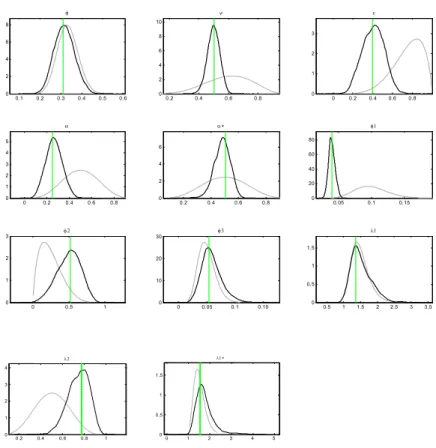
We also estimated a subset of deep parameters assuming the rule-of-thumb proportion to be 0.6 (we obtained similar IRFs as from the estimated VAR). Other deep parameters (relatively less important) were calibrated because otherwise the parameter space of the log-likelihood function becomes too large. In total, we estimated 11 deep parameters using Bayesian techniques, which resulted in all of them showing well-behaved posterior distributions (narrower than before and centered around the state).