WORKING PAPER-REIHE DER AK WIEN
DRIVERS OF WEALTH INEQUALITY IN EURO AREA COUNTRIES
137
Sebastian Leitner
MATERIALIEN ZU WIRTSCHAFT UND GESELLSCHAFT
Materialien zu Wirtschaft und Gesellschaft Nr. 137 Working Paper-Reihe der AK-Wien
Herausgegeben von der Abteilung Wirtschaftswissenschaft und Statistik der Kammer für Arbeiter und Angestellte
für Wien
Drivers of wealth inequality in euro area countries
Sebastian Leitner
Februar 2015
Die in den Materialien zu Wirtschaft und Gesellschaft veröffentlichten Artikel geben nicht unbedingt die
Meinung der AK wieder.
Die Deutsche Bibliothek – CIP-Einheitsaufnahme
Ein Titeldatensatz für diese Publikation ist bei der Deutschen Bibliothek erhältlich.
ISBN 978-3-7063-0528-0
Kammer für Arbeiter und Angestellte für Wien
A-1041 Wien, Prinz-Eugen-Straße 20-22, Tel: (01) 501 65, DW 2283
Drivers of wealth inequality in euro area countries
The effect of inheritance and gifts on gross, net and real estate asset distribution analysed by applying the Shapley value approach to decomposition
February 2015 by Sebastian Leitner†°
Abstract:
This paper investigates the sources of inequality in household gross, net and real estate gross wealth across eight euro area countries applying the Shapley value approach to decomposition. The research draws on micro data from the Eurosystem Household Finance and Consumption Survey 2010. Dispersion in bequests and inter vivos transfers obtained by households are found to have a remarkable effect on wealth inequality that is stronger than the one of income differences. In South European countries, Austria and Germany the contribution to wealth inequality of real and financial assets inherited or received as gifts attains 30% to 40%. Nevertheless, also the distribution of household characteristics (age, education, size, number of adults and children in the household, marital status) within countries shapes the observed wealth dispersion.
JEL classification: D31, D63, O52, O57
Keywords: Inequality, Wealth Distribution, Decomposition Analysis, Inheritance, Inter vivos transfers, Income Distribution, Europe
Research was financed by the Austrian Chamber of Labour.
† The Vienna Institute for International Economic Studies (wiiw); Rahlgasse 3, 1060 Vienna, Austria;
Email: [email protected]
° The author wishes to thank Stefan Jestl and Mario Holzner for helpful comments and suggestions.
Kurzfassung:
In der vorliegenden Studie werden die Ursachen für die Ungleichheit von Brutto-, Netto- und Immobilienvermögensbeständen in acht Ländern der Eurozone untersucht. Die Analyse basiert auf Mikrodaten des Eurosystem Household Finance and Consumption Survey (HFCS 2010) und wird mittels der sogenannten Shapley-Wert-Dekompositionsmethode durchgeführt. Die
Forschungsergebnisse zeigen, dass Erbschaften und Schenkungen einen beachtlichen Effekt auf die gemessene Vermögensungleichheit haben; dieser ist stärker als der Einfluss vorhandener
Einkommensdifferenzen. Ererbte Sach- und Finanzwerte tragen zwischen 30% und 40% zur gesamten gemessenen Vermögensungleichheit in Österreich, Deutschland und manchen Südeuropäischen Ländern bei; Haushaltseinkommen nur 20% oder weniger. Gleichwohl prägt auch die Verteilung anderer sozioökonomischer Charakteristika der Haushalte innerhalb der Länder (Alter, Bildungsstand, Haushaltsgröße, Anzahl Erwachsener sowie Kinder im Haushalt und Familienstand) die beobachtete Vermögensverteilung.
1
Introduction
The topic of household wealth holdings and their distribution is being discussed intensively in the recent literature. One of the reasons for this is the increase of accumulated private wealth in relation to the national income in the affluent industrialised economies from the 1950s onwards (Piketty, 2014). Before, in the course of the first half of the 20th century, two world wars and the economic depression in between effected a remarkable capital destruction and thus a slump in the ratio of wealth to national income. In addition to this development, in most OECD countries inequality of income rose from the 1980s onwards (see e.g. OECD, 2010). From research based on national surveys we can also conclude that at least in a couple of countries analysed also wealth inequality started to increase from at least the mid-1980s. For the United States this is detected by e.g. Wolff (2007, 2010) and Kennickell (2003), for Canada by Morissette et al. (2003), for Sweden by Klevmarken (2004), for Finland by Jäntii (2006), for Italy by Brandolini et al. (2004), for Germany by Hauser and Stein (2003) and for France by Piketty (2014). Overviews on developments in wealth inequality on the national level can also be found in Jäntti and Sierminska (2007) and Bonesmo Fredriksen (2012).
Another reason for the increased interest in research on household wealth is that most recently micro data have become available that allow to compare wealth holdings and inequality across countries, first via the Luxembourg Wealth Study Database and more recently in the Eurosystem Household Finance and Consumption Survey (HFCS).
The present paper aims to analyse the sources of wealth inequality on the national level for various euro area countries and to compare those sources. Our assumption is that the accumulation of wealth stocks by households is facilitated by the receipt of bequests or gifts (mostly of ancestors).
Thus wealth inequality of one generation can be passed on to the following, which over longer periods of time may result in an increase in inequality of wealth within a society. As is laid down by Piketty and Zucman (2014) in Germany and France the ratio of bequests and gifts to the total stock of wealth has increased considerably, while remaining rather stable in the United Kingdom and Sweden.
In principle, households build up wealth stocks in two ways. Either they save out of their income from employment or self-employment or out of financial sources. The second way, important for many households, is to receive bequests or gifts and save them instead of using the assets for consumptive purposes. A third form, which however cannot be dealt with in this paper, is that the assets owned appreciate in real terms. In our paper we are interested in the process of households’
building up of wealth stocks via the first two processes and the respective inequality in asset holdings that results therefrom. In order to detect the sources of wealth inequality across countries we apply a decomposition methodology based on the Shapley value approach to the inequality measure used most frequently in the literature – the Gini index. This decomposition method allows for an assessment of the relative importance of explanatory factors for inequality.
The paper is organised as follows: Section 2 provides a brief discussion of the literature on developments of household wealth inequality, the effects of inheritance and inter vivos transfers and on decomposition methods used to analyse income and wealth inequality. Section 3 discusses the most relevant aspects of the data used (sources, measurement issues and definitions) and Section 4 introduces the concept of the Shapley value approach to decomposition, discussing the way we apply this method. Section 5 presents the empirical results of the analysis for inequality in gross and net wealth stocks and real estate gross wealth. Section 6 concludes.
2
Literature review
Evidence shows that wealth is less equally distributed than income. The reasons for this are manifold (for an overview see e.g. Davies and Shorrocks, 2000). Apart from an obvious existing variation in structural differences in terms of skills or fortune, and preferences in terms of saving and consumption behaviour etc. which renders people more or less capable of making a fortune, wealth inequality is driven by two main sources. First, the accumulation of wealth takes time if achieved via saving out of income and investment of funds; hence over the lifecycle households have the chance to build up stocks of assets, which are then used as a tool to secure consumption levels in times of negative income shocks or lowered income levels after retirement. Thus we would expect a dispersion of wealth stocks according to age groups in the society. The second reason for wealth inequality is to be found in the intergenerational transmission of wealth via bequests or inter vivos gifts. The results of the research on which of the two reasons is more important in shaping the existing wealth distribution differ remarkably. While Kotlikoff and Summers (1981, 1988) claimed that for the United States between 46% and 80% of household wealth can be attributed to inheritance (including gifts), Modigliani (1988) and Smith (1999) argue that only about 20% can be interpreted as such. Wolff (2002) estimates a share of 19-35%, while Gale and Scholtz (1994) assume that 50% of the wealth is made up of transfers from ancestors. Davies and Shorrocks (2000) believe that a reasonable rough estimate would be to assume the share of gifts and bequests in total wealth to amount to 35% to 45% in the United States. For Sweden Klevmarken (2004) presents a range of 10-20%, while for the UK an early estimation for 1973 amounts to 25% including only a limited range of inter vivos transfers (Royal Commission on the Distribution of Income and Wealth, 1977). The large divergence in the results of the cited studies stems inter alia from different views on which investments in the offspring (e.g. education) can be interpreted as inter vivos transfers and depends on the degree of capitalisation of inherited wealth.
The literature on the links between wealth accumulation and inheritance claims that the distribution of household wealth strongly depends on the patterns of bequests or gifts made before the death of the bequeathers to their offspring. For the United States Wolff and Gittleman (2011) and for France Arrondel et al. (2001) find that these wealth transfers are more concentrated than total wealth holdings in those countries.
In this paper we apply a decomposition approach, an analysis which has already a long tradition in the literature; to be more precise, we perform a decomposition by subgroups, including also groups of households with different levels of inheritance and income received. Early applications and methodological analysis on income sources have been delivered by e.g. Cowell (1980), Fei et al. (1979), Fields (1979) and Shorrocks (1982). On decomposition by population subgroups, Theil (1972) was probably the first to deliver methods and was followed by Bourguignon (1979), Shorrocks (1980, 1984) and Foster and Shneyerov (1996a, 1996b). However, regression-based methods such as the Shapley value approach were introduced somewhat later in the inequality literature starting with Shorrocks (1999 – reprint 2013). Further applications have been done by Fields and Yoo (2000), Morduch and Sicular (2002), Sastre and Trannoy (2002), Fields (2003), Wan (2004), Molini and Wan (2008) and Gunatilaka and Chotikapanich (2009); for a critical review see e.g. Cowell and Fiorio (2009) and Chantreuil and Trannoy (2013). Israeli (2007) shows how the Shapley approach is related to the method proposed by Fields
3
(2003), who decomposes the R² of the underlying regression instead of the resulting inequality measure.
The most important advantage of the Shapley value approach is that it takes the potential correlation amongst all regressors into account. More recently Chernozhukov et al. (2009) and Fortin et al. (2010) have introduced applications of decomposition analysis based on counterfactual analysis.
Most decomposition analyses have been performed on income inequality and its development over time;
only some applications have been done so far on wealth inequality. Wolff (2002) decomposes the coefficient of variation in order to analyse the effect of bequests on wealth inequality in the United States in the 1990s. Brandolini et al. (2004) assess for Italy and Azpitarte (2008) for Spain that wealth inequality is mostly driven by inequality in real assets in contrast to financial wealth assets. Sierminska et al. (2008) study the drivers of the gender wealth gap in Germany, while Lindner (2011) decomposes income and wealth inequality in Austria by components. Sierminska and Doorly (2012) analyse the participation and level decision for chosen assets across households and show that household characteristics explain a sizeable portion of both wealth participation and levels in a sample of European countries, the United States and Canada.
Data
The data for the analysis presented in this paper are drawn from the Eurosystem Household Finance and Consumption Survey for the year 2010 (HFCS 2010), which was conducted in 15 euro area countries1, while Estonia and Ireland are not included. A detailed description of the methodology of the survey is presented by the European Central Bank (2013). The HFCS provides data on gross and net wealth holdings of households and their components and socioeconomic characteristics for the households and their individual members. Moreover, it covers data on inheritance and gifts received and gross income.
Interpreting results in cross-country comparisons of wealth inequality should be done cautiously. As discussed by e.g. Fessler et al. (2013) and Tiefensee and Grabka (2014), there are several aspects of potential methodological constraints regarding cross‐country comparability due to non-harmonisation of sampling frames, sample sizes, survey modes, oversampling of top wealth households, reference periods, weighting or imputation methods applied and variations in initial response rates by countries.
Nevertheless, as emphasised by Tiefensee and Grabka (2014), ’the HFCS is still the best dataset for cross- country comparisons of wealth levels and inequality in the Euro area and it is definitely a first (big) step into the right direction’. The HFCS data offer in order to correct for item non-response five different multiple imputations. We take these imputations into account in our estimation analysis by using Rubin’s Rule. Moreover unit non-response is accounted for in the HFCS data by providing 1000 replicate weights, which are all used in our estimations.
In our analysis we decompose three different variables depicting wealth holdings of households: gross wealth (total household assets excluding public and occupational pension wealth), net wealth (gross wealth minus total outstanding household liabilities) and real estate wealth. As explanatory variables we apply first total household gross income and five different types of inheritances and gifts (household main residence, further dwellings, land, business and the sum of other assets) received by all household
1 The HFCS 2010 was conducted in Austria, Belgium, Cyprus, Finland, France, Germany, Greece, Italy, Luxembourg, Malta, the Netherlands, Portugal, Spain, the Slovak Republic and Slovenia.
4
members. Obviously, the net income of households would be a better measure to assess the potential of households to save out of their income; moreover, present income may not be the best predictor of income flows accrued by individuals in their previous (working) life; however, this information is so far not available in the HFCS. In the HFCS 2010 the reference person is asked to provide information on whether the main household residence, if owned, was inherited or a gift. Furthermore, information is collected on up to three inheritances or substantial gifts from someone who is not a part of the current household.
Since in the case of Finland no data were provided on inheritances, in the case of France no information was available on the way of acquisition of the household main residence (which could be a bequest or gift) and for Italy and the Netherlands only 2.1% and 6.7% of all households provided information on inheritances (and gifts) received (see Table 1) we had to exclude those four countries from the analysis.
Malta could not be included in the analysis either due to multiple data problems. In general, inheritance data have to be interpreted cautiously since inheritances are notoriously under-reported in wealth surveys. Particularly the rate of refusing to answer questions concerning inheritances rises in line with the wealth holdings of households (Fessler et al., 2013). Most probably this results in an underestimation of wealth inequality.
It should be pointed out that bequests and gifts acquired in the past are not automatically part of the actual present wealth stock. In the period between acquisition and the time of the interview of the survey, assets may have been used not only for the accumulation of the wealth stock of the household but e.g. also for consumption purposes or inter-household transfers. Thus a regression of wealth stocks on wealth transfers received is not a performance of explaining the total sum of wealth by its parts.
In addition to the value of the property at the time of acquisition (by way of inheritance or gift) information is collected on the date of acquisition. In order to make the assets inherited or acquired as gifts comparable both with each other in households and between households, we have to calculate the present value of the assets. The problem is dealt with in different ways in the literature; the assumptions made differ between a real depreciation (by leaving the nominal value of the acquired asset unchanged) and an appreciation of up to 3 per cent annually. For the lack of information on actual appreciation we resort to the conservative method applied by e.g. Fessler et al. (2008a, 2008b, 2013) assuming the retention of the real value of the asset by appreciation, using the annual national consumer price index (CPI). The data were provided by the AMECO database from 1960 onwards for all countries except for the Slovak Republic and Slovenia. Thus we excluded those two countries from the analysis as well. For assets acquired before 1960 we have to assume no increase in value up to 1960. Of those households having received inheritances and gifts, 1.5% acquired them before 1960 (unweighted average over country shares). Concerning the application of the CPI for the calculation of the present value of the assets inherited or received as gifts we do not differentiate between different kinds of assets since households could swap between asset types. We use the information of asset types acquired however for one differentiation: In the case of land, dwellings apart from the household main residence and businesses acquired we assume that households have a relatively higher incentive to keep those assets and further invest in them and that those assets appreciate with an interest rate exceeding the CPI (the applied appreciation rate for bequests and gifts) resulting in higher wealth stocks of households having inherited those assets. Thus the information on the present value of businesses (also farms are included), land and dwellings acquired via inheritance (or as gift) were used as separate explanatory variables apart from further assets inherited (or received as gifts). Some information which was used as an additional explanatory variable was not collected in all euro area countries. This was e.g. the case for the question of
5
expectations on the receipt of a substantial gift or inheritance in the future and information on the country of birth of the reference person.
Furthermore we use socioeconomic characteristics as control variables. For this we employed personal characteristics of the household members in order to construct variables for the household level. These are the household level of educational attainment, the average age of adult household members (being more than 19 years of age), the household size, i.e. the number of adults and children in the household.
Moreover, we used dummies for the country of birth of the household reference person (survey or foreign country) and the marital status of the household reference person (being single, married, widowed, divorced or living in a consensual union on a legal basis). The household level of educational attainment is calculated as the average attainment level (expressed in average years of schooling needed to attain the education level stated for the individual household members) of all household members above the age of 16 and no longer in education (and thus potentially available for the labour market). The use of socioeconomic characteristics is particularly important in the case of cross-country comparisons since differences in household structures have a substantial effect on the measured summary statistics of wealth distribution in the euro area (see e.g. Fessler et al., 2014). For instance, we expect that households with more members, those with higher average education levels and with higher average age of the household members tend to possess higher stocks of gross and net wealth.
Methodology
The advantage of a regression-based approach is that the relative importance of many variables and groups of them to explain inequality (socioeconomic characteristics of individuals or households such as age, gender, educational attainment, employment status, but also decisive monetary values such as income, etc.) is taken into account simultaneously. Thus, the regression approach (step 1) allows assessing the importance of each of these explanatory variables conditional on all other variables for any dimension of inequality considered (in our case stocks of household net, gross and gross real estate wealth). The Shapley value approach (step 2) then further allows calculating the contribution of each of these explanatory variables to the respective inequality measure.
The Shapley value approach can be illustrated by using a simple example with three explanatory variables. We first regress individual wealth levels y on these explanatory variables
x
i (i1,2,3),
0 1x1 2x2 3x3
y ,
where denotes the error term. The predicted wealth level is then given by ˆ .
ˆ ˆ
ˆ123 ˆ0 1x1 2x2 3x3 y
This predicted value is then used to calculate the Gini coefficient
G ˆ
1230 , where subscripts denote the variables included. In the first round we then eliminate one variable and calculate the predicted wealth levels yˆ 23,yˆ 13 and yˆ 12. The corresponding Gini coefficients are then given by Gˆ 123,Gˆ 131 and Gˆ 121 respectively. Analogously, in a second round we eliminate two variables, thus calculating6
1,ˆ 2
ˆ y
y and yˆ 3 . The resulting Gini coefficients are
G ˆ
12, G ˆ
22 and Gˆ 32 . The final round would then be to include the constant only; the resulting Gini coefficient would thus beG ˆ
3 0 .
The marginal contributions are then calculated using the Gini coefficients. The first round marginal contributions for each variable are
C
1(1) G ˆ
(1230) G ˆ
(231) ,C
2(1) G ˆ
(1230) G ˆ
(131) and (121) )
0 ( 123 )
1 (
3
G ˆ G ˆ
C
.The marginal contributions in the second round of the first variable are given by
(22) )
1 ( 12 ) 1 , 2 (
1
G ˆ G ˆ
C
andC
1(2,2) G ˆ
(131) G ˆ
(32)The average of these contributions is the marginal contribution of the first variable in the second round, i.e.
1 2,2
1 , 2 1 )
2 (
1 2
1 C C
C . Similarly we calculate
C
2 2 and C3 2 . The third round contribution is given by (12)) 3 ( ) 2 (
1 ) 3 (
1
G ˆ G ˆ G ˆ
C
asG ˆ
(3) 0
and analogously for C2(3) Gˆ (22) and C3(3) Gˆ (32).Finally, averaging the marginal contributions of each variable over all rounds j 1,2,3 results in the total marginal effect of each variable, i.e.
1 2 3
3 1
j j
j
j C C C
C .
The proportion of inequality not explained is then given by
(1230)
Gˆ G
CR .
The approach can easily be extended to any number of explanatory factors and to other inequality measures. However, since the number of combinations and thus Gini coefficients to be calculated grows exponentially with the number of variables, in practice is it necessary to combine the variables to seven or eight explanatory factors in order to keep the necessary computing time tolerable. In our case we included in the explanatory factor inheritance the effect of the individual types of bequests and gifts and the effect of expected inheritance; the factor household age includes the variable household age and household age2, household structure includes the effect of both the variables number of adults and number of children and the explanatory factor marital status comprises the effect of all three dummy variables for single, widowed and divorced reference persons of households (comparing their wealth holdings with those of reference persons being married or living in a consensual union).
Wan (2002) points to the fact that the presence of a negative constant in the regression equation may lead to negative predicted individual income levels. In that case the calculation of a Gini coefficient and thus the contributions of individual variables to overall inequality would be impossible. To overcome this pitfall he shows in Wan (2004) that different model specifications can be used for the underlying estimated income (in our case wealth) generating function, delivering
7
moreover better log-likelihood values than the linear estimation model. Following his approach, we choose for the analysis in this paper a semilog model:
0 1 1 2 2 3 3
lny x x x .
Since the distribution of wealth data is not only highly skewed but net wealth data also comprise, due to outstanding debts of households, negative and zero values we cannot apply a logarithmic transformation of the data but resort to a transformation often used in the literature on wealth stocks (see e.g. Burbidge et al., 1988; MacKinnon and Magee, 1990; Pence, 2006; Schneebaum et al., 2014) – the inverse hyperbolic sine transformation (IHS):
( i) ln i i2 1
i IHS W W W
y .
This transformation is used not only for the wealth stocks but also the calculated sums of inheritances and gifts and the income of households since both can also feature zero and the latter for self-employed income also negative values. Since we are not interested in the decomposition of the log of net wealth, but net wealth in nominal terms, for the second step of the decomposition analysis we have to take the antilog of the above model resulting in
e e e e
e
e
lnyi
0
! x1i
2 x2i
3 x3i
,which in our case after the above-described IHS transformation results in
e e e e
e W
W
yi i i2 1 0 ! x1i 2 x2i 3 x3i .
The simple advantage of this model is that the constant e0 is now a positive scalar which does not influence the magnitude of the calculated Gini coefficient. The elimination procedure as described above however remains unchanged. As one can see, we approximate the level of wealth inequality with the level of Wi Wi2 1. This would only be problematic if we had a large number of negative predicted values. However, based on the wealth generating function stemming from our regressions, this is not the case and the inequality levels calculated are the same for Wi Wi2 1 and Wi.
Empirical results
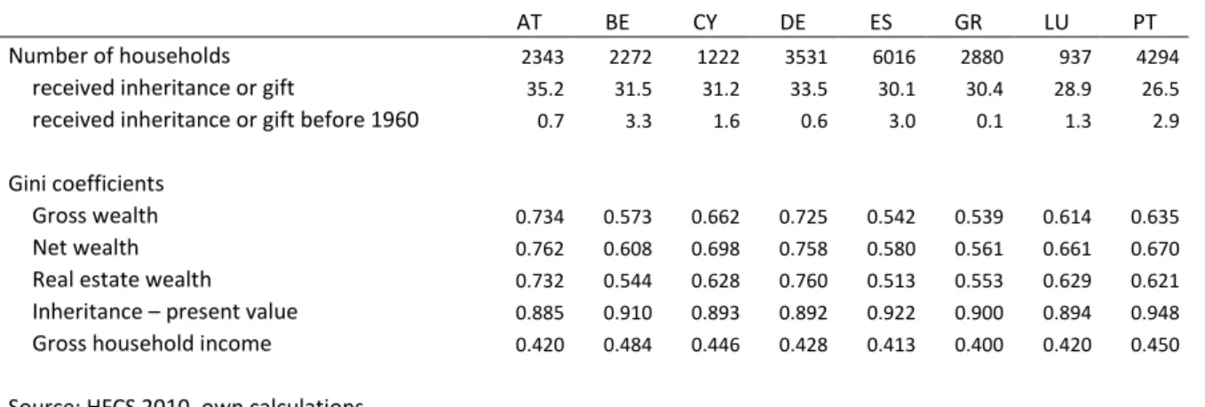
In order to describe the situation of wealth distribution in the analysed countries, we start by taking a look at the inequality of income and wealth holdings across countries. Table 1 presents the Gini indices of wealth assets of households. We can observe that gross and net wealth as well as real estate wealth are distributed more unequally compared to household gross income. Moreover, the Gini indices for wealth holdings are much higher in Austria and Germany, while lowest in Spain, Greece and Belgium. Bequests and gifts at present value are even more unequally distributed than net wealth. Taking into account the underreporting of inheritances, the inequality of bequests may
8
be even higher. This is an effect of the relatively low rates of households having acquired an inheritance (or substantial gift) up to the date of the survey. In Portugal only an estimated 26.5% of all households received bequests, while in Austria the share is 35.2%.
Table 1: Descriptive statistics of inheritance and gifts, wealth stocks and household income
AT BE CY DE ES GR LU PT
Number of households 2343 2272 1222 3531 6016 2880 937 4294
received inheritance or gift 35.2 31.5 31.2 33.5 30.1 30.4 28.9 26.5
received inheritance or gift before 1960 0.7 3.3 1.6 0.6 3.0 0.1 1.3 2.9 Gini coefficients
Gross wealth 0.734 0.573 0.662 0.725 0.542 0.539 0.614 0.635
Net wealth 0.762 0.608 0.698 0.758 0.580 0.561 0.661 0.670
Real estate wealth 0.732 0.544 0.628 0.760 0.513 0.553 0.629 0.621
Inheritance – present value 0.885 0.910 0.893 0.892 0.922 0.900 0.894 0.948 Gross household income 0.420 0.484 0.446 0.428 0.413 0.400 0.420 0.450 Source: HFCS 2010, own calculations.
Regression analysis
Following the above-described approach of the Shapley value decomposition we first regress the IHS-transformed gross wealth assets of the household on the explanatory variables. In our case these are the IHS-transformed present values of five different types of bequests and gifts, first the household main residence (HMR), dwellings (excluding the HMR), land, businesses and the sum of other types of assets, a dummy for the expectation of future substantial bequests or gifts, the IHS-transformed gross household income and a set of socioeconomic characteristics. These are the average age of the household members (and the square of this variable), the average education level attained by those household members being more than 16 years of age and no longer in education (and thus potentially available for the labour market) and the number of adults and children in the household. Moreover, we apply dummies for the country of birth of the reference person of the household and marital states respectively. We expect wealth holdings of households to increase conditionally on amounts of inheritances (and substantial gifts) acquired and household gross income respectively.
The results presented in Table 2 below show that in general the coefficients are of the expected signs in the regressions and significant for a large part of the explanatory variables in most countries. The explained part of the variance amounts to 34% on average (unweighted over countries) as shown by the R². For most inherited asset types the positive conditional correlation with gross wealth stocks is highest for Germany and Austria. An interesting result is that the incidence of having inherited a business alters the conditional accumulation behaviour (more precise results) of households not in all countries significantly, i.e. in Austria and Luxembourg. The higher the average age of the household, the more the members had time to accumulate wealth holdings. Coefficients for age and age² show that household gross wealth rises with increasing average age of the (adult) household members. For most countries on average the conditional peak of wealth holdings is reached at about 55 years (average age of adult household members). Households with higher average education levels hold conditionally higher gross wealth stocks. In general larger households seem to have the possibility to
9
accumulate higher wealth stocks; no significant results however are available for the number of children in the household.
Table 2: OLS estimations predicting IHS-transformed household gross wealth stocks
Independent Variables AT BE CY DE ES GR LU PT
Inheritance (IHS) 0.133*** 0.046*** 0.067*** 0.113*** 0.042*** 0.092*** 0.065*** 0.074***
Household main residence (0.008) (0.017) (0.017) (0.010) (0.007) (0.006) (0.022) (0.010) Inheritance (IHS) 0.074*** 0.071*** 0.037* 0.082*** 0.057*** 0.003 0.031** 0.050***
Dwellings excl. HH main res. (0.013) (0.011) (0.021) (0.011) (0.006) (0.017) (0.013) (0.011) Inheritance (IHS) 0.104*** 0.052*** 0.061*** 0.098*** 0.055*** 0.053** 0.037* 0.095***
Land (0.013) (0.013) (0.014) (0.017) (0.009) (0.026) (0.019) (0.009)
Inheritance (IHS) 0.054 0.098*** 0.141*** 0.121*** 0.067*** 0.208*** 0.021 0.084**
Business (0.038) (0.016) (0.047) (0.034) (0.014) (0.051) (0.074) (0.034) Inheritance (IHS) 0.053*** 0.037*** 0.080*** 0.074*** 0.042*** 0.070*** 0.031** 0.042***
Other assets (0.012) (0.009) (0.022) (0.010) (0.008) (0.024) (0.014) (0.012) Expectation of substantial 0.311** 0.320** -0.211 0.561*** . 0.279* 0.158 0.493***
gift or inheritance (0.148) (0.129) (0.281) (0.131) . (0.156) (0.173) (0.094) Gross income (IHS) 0.662*** 0.366*** 0.341*** 0.880*** 0.307*** 0.339*** 0.330* 0.292***
(0.232) (0.075) (0.111) (0.138) (0.056) (0.112) (0.195) (0.058) Household age 0.106*** 0.110*** 0.146** 0.002 0.113*** 0.243*** 0.013 0.082***
(average of adults) (0.019) (0.023) (0.064) (0.033) (0.022) (0.034) (0.040) (0.022) Household age2 -0.001*** -0.001*** -0.002** 0.000 -0.001*** -0.002*** 0.000 -0.001***
(0.000) (0.000) (0.001) (0.000) (0.000) (0.000) (0.000) (0.000) Household education 0.130*** 0.134*** 0.110*** 0.200*** 0.109*** 0.086*** 0.167*** 0.180***
(average of years of adults) (0.031) (0.018) (0.033) (0.028) (0.011) (0.021) (0.024) (0.012) Number of adults 0.397*** 0.462*** 0.120 0.431*** 0.093 0.315*** 0.515*** 0.076
(0.106) (0.080) (0.114) (0.132) (0.069) (0.073) (0.116) (0.065)
Number of children 0.034 -0.115 0.023 0.000 0.016 0.093 0.033 -0.132**
(0.064) (0.106) (0.083) (0.080) (0.069) (0.071) (0.088) (0.064) Reference person: -1.040*** -1.638*** -0.293 -0.690*** . . 0.521*** -0.639***
Foreign country of birth (0.236) (0.293) (0.216) (0.181) . . (0.168) (0.217) Reference person: single -0.548*** -0.566*** -0.991*** -0.570*** -0.736*** -0.565*** -0.834*** -1.504***
(0.152) (0.153) (0.383) (0.203) (0.141) (0.118) (0.225) (0.221) Reference person: widowed -0.606*** -0.334 -1.765*** -0.355 -0.119 -0.367* 0.356 -0.873***
(0.198) (0.210) (0.582) (0.265) (0.142) (0.217) (0.275) (0.165) Reference person: divorced -0.836*** -0.615*** -0.991** -0.922*** -0.745*** -0.915*** -0.259 -1.193***
(0.174) (0.193) (0.448) (0.244) (0.173) (0.246) (0.249) (0.208) Constant -2.262 0.769 4.191** -3.268** 4.454*** -0.453 5.413*** 3.947***
(2.405) (0.968) (1.755) (1.476) (0.770) (1.537) (1.851) (0.756)
R2+) 0.408 0.330 0.349 0.444 0.344 0.233 0.387 0.230
Observations 2,341 2,274 1,032 3,498 6,192 2,878 950 4,227
Standard errors in parentheses
*** p<0.01, ** p<0.05, * p<0.1 +) R2 using Fisher's z over imputed data Source: HFCS 2010, own calculations.
As expected, those households where the reference person’s country of birth is foreign face lower wealth stocks (except for Luxembourg); households where the reference person is married or lives in a consensual union have conditionally higher wealth stocks compared to all other households. For completeness we should also mention here that in an earlier version of the regression model we included
10
also the gender of the reference person as an explanatory variable and the share of female members in households. However, the results were non-significant.
Table 3: OLS estimations predicting IHS transformed household net wealth stocks
Independent Variables AT BE CY DE ES GR LU PT
Inheritance (IHS) 0.200*** 0.064*** 0.092* 0.169*** 0.087*** 0.148*** 0.112*** 0.098***
Household main residence (0.021) (0.021) (0.047) (0.020) (0.012) (0.010) (0.034) (0.013) Inheritance (IHS) 0.078** 0.078*** 0.085** 0.107*** 0.085*** 0.039 0.021 0.071***
Dwellings exl. HH main resid. (0.033) (0.019) (0.036) (0.022) (0.013) (0.025) (0.034) (0.016) Inheritance (IHS) 0.165*** 0.063*** 0.114*** 0.137*** 0.081*** -0.015 0.072** 0.130***
Land (0.028) (0.019) (0.028) (0.045) (0.013) (0.084) (0.032) (0.015)
Inheritance (IHS) -0.032 0.101*** 0.207*** 0.165*** 0.114*** 0.279*** 0.043 0.150***
Business (0.118) (0.027) (0.071) (0.060) (0.017) (0.075) (0.098) (0.037) Inheritance (IHS) 0.060** 0.036* 0.051 0.138*** 0.064*** 0.053 0.069*** 0.062***
Other assets (0.027) (0.021) (0.069) (0.022) (0.017) (0.042) (0.023) (0.024) Expectation of substantial 0.874** 0.174 0.607 1.453*** . 0.483 0.213 0.841***
gift or inheritance (0.432) (0.256) (0.513) (0.295) . (0.319) (0.424) (0.191) Gross income (IHS) 0.992** 0.398*** 0.298 1.178*** 0.209** 0.353*** 0.395 0.238***
(0.441) (0.093) (0.188) (0.243) (0.085) (0.130) (0.253) (0.061) Household age 0.158*** 0.192*** 0.106 0.035 0.323*** 0.224*** 0.160* 0.195***
(average of adults) (0.052) (0.049) (0.090) (0.068) (0.062) (0.042) (0.091) (0.040) Household age2 -0.001** -0.001*** -0.001 0.000 -0.002*** -0.002*** -0.001 -0.001***
(0.000) (0.000) (0.001) (0.001) (0.001) (0.000) (0.001) (0.000) Household education 0.230*** 0.162*** 0.186*** 0.273*** 0.164*** 0.125*** 0.250*** 0.231***
(average of years of adults) (0.067) (0.028) (0.060) (0.058) (0.026) (0.030) (0.050) (0.022) Number of adults 0.474** 0.673*** -0.023 0.792*** 0.166 0.473*** 0.672*** 0.314***
(0.213) (0.126) (0.316) (0.276) (0.148) (0.132) (0.251) (0.110) Number of children -0.488* -0.224 -0.180 0.151 -0.202 0.103 -0.403* -0.172 (0.255) (0.164) (0.156) (0.214) (0.237) (0.155) (0.242) (0.115) Reference person: -1.701*** -2.166*** -0.035 -0.716* . . 0.749* -0.687*
Foreign country of birth (0.607) (0.538) (0.580) (0.416) . . (0.397) (0.384) Reference person: single -0.503 -0.271 -2.330** -0.090 -1.209*** -0.351 -0.952* -1.519***
(0.403) (0.298) (0.985) (0.492) (0.368) (0.220) (0.512) (0.324) Reference person: widowed -0.365 -0.132 -2.648** -0.072 -0.073 -0.029 0.282 -0.740***
(0.346) (0.338) (1.040) (0.456) (0.445) (0.246) (0.699) (0.216) Reference person: divorced -1.526*** -0.428 -2.490** -2.090*** -1.238*** -1.681*** -0.627 -1.834***
(0.465) (0.328) (1.015) (0.615) (0.400) (0.394) (0.726) (0.447) Constant -11.026** -3.920** 3.515 -12.25*** -2.102 -2.379 -1.723 -0.961 (5.031) (1.682) (2.742) (2.960) (2.037) (1.654) (3.226) (1.355)
R2+) 0.204 0.206 0.120 0.244 0.203 0.208 0.150 0.209
Observations 2,341 2,274 1,032 3,498 6,192 2,878 950 4,387
Standard errors in parentheses
*** p<0.01, ** p<0.05, * p<0.1 +) R2 using Fisher's z over imputed data Source: HFCS 2010, own calculations.
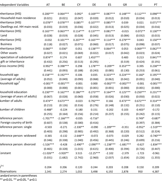
In addition to gross wealth holdings of households we also regress net wealth holdings on the above- described explanatory variables. The results reported in Table 3 above are similar to those with respect to household gross wealth. Coefficient signs remain in general the same, whilst the share of the explained variance drops to an R² of some 19%. This is no surprise since the underlying decisions of households to borrow money for private or business purposes are even more influenced by reasons difficult to be
11
described with the information available from the HFCS. In general, the signs of the coefficients do not change and remain significant in almost all cases. The size of the coefficients increases for almost all variables throughout the majority of countries, particularly for inheritance (and gifts) and household income, but also in the case of household age, education level, number of adults in the household and foreign country of birth. For single and widowed reference person the coefficients become insignificant in a couple of countries while for households with divorced reference persons the value of the negative coefficient rises in most countries.
Table 4: OLS estimations predicting IHS-transformed household real estate gross wealth stocks
Independent Variables AT BE CY DE ES GR LU PT
Inheritance (IHS) 0.486*** 0.196*** 0.200*** 0.420*** 0.140*** 0.237*** 0.153*** 0.242***
Household main residence (0.020) (0.033) (0.029) (0.021) (0.013) (0.011) (0.049) (0.016) Inheritance (IHS) 0.214*** 0.181*** 0.074** 0.238*** 0.106*** 0.041 0.076* 0.075***
Dwellings exl. HH main resid. (0.044) (0.022) (0.036) (0.033) (0.015) (0.036) (0.041) (0.029) Inheritance (IHS) 0.316*** 0.142*** 0.130*** 0.295*** 0.105*** 0.114*** 0.118*** 0.241***
Land (0.043) (0.031) (0.032) (0.041) (0.018) (0.043) (0.044) (0.023)
Inheritance (IHS) -0.085 -0.004 0.182*** 0.080 0.043 0.325*** 0.078 0.068 Business (0.129) (0.051) (0.069) (0.108) (0.043) (0.070) (0.171) (0.138) Inheritance (IHS) 0.148*** 0.043 0.154*** 0.149*** 0.083*** 0.157*** 0.096*** 0.054 Other assets (0.037) (0.029) (0.051) (0.028) (0.018) (0.049) (0.036) (0.037) Expectation of substantial -0.842* 0.305 -0.773 -0.490 . -0.119 0.059 0.653**
gift or inheritance (0.435) (0.349) (0.544) (0.442) . (0.383) (0.498) (0.270) Gross income (IHS) 0.778* 0.472*** 0.683*** 1.066*** 0.462*** 0.295*** 0.683 0.306***
(0.434) (0.114) (0.212) (0.251) (0.111) (0.096) (0.434) (0.081) Household age 0.287*** 0.318*** 0.117 0.290*** 0.319*** 0.517*** 0.235** 0.364***
(average of adults) (0.046) (0.066) (0.100) (0.061) (0.051) (0.046) (0.104) (0.060) Household age2 -0.002*** -0.002*** -0.001 -0.002*** -0.002*** -0.004*** -0.001 -0.003***
(0.000) (0.001) (0.001) (0.001) (0.000) (0.000) (0.001) (0.001) Household education 0.184** 0.277*** 0.143*** 0.262*** 0.136*** 0.088** 0.294*** 0.271***
(average of years of adults) (0.075) (0.043) (0.055) (0.054) (0.025) (0.039) (0.062) (0.031) Number of adults 0.974*** 1.261*** 0.089 1.056*** 0.102 0.904*** 1.127*** 0.441***
(0.262) (0.211) (0.243) (0.244) (0.164) (0.129) (0.310) (0.123)
Number of children 0.102 0.127 0.155 0.174 0.151 0.389*** 0.132 0.016
(0.184) (0.176) (0.222) (0.189) (0.177) (0.136) (0.228) (0.146) Reference person: -1.252*** -2.702*** 0.282 -0.906** . . 2.201*** -1.571***
Foreign country of birth (0.424) (0.577) (0.572) (0.381) . . (0.507) (0.496) Reference person: single -1.299*** -2.174*** -1.650* -2.092*** -1.735*** -1.161*** -1.914*** -2.575***
(0.386) (0.470) (0.886) (0.427) (0.327) (0.266) (0.610) (0.368) Reference person: widowed -1.865*** -0.046 -2.820*** 0.095 -0.317 0.158 1.163 -0.736**
(0.556) (0.500) (1.036) (0.491) (0.347) (0.335) (0.813) (0.319) Reference person: divorced -2.227*** -2.099*** -1.555* -2.041*** -1.432*** -1.085** -1.254* -1.460***
(0.472) (0.505) (0.797) (0.427) (0.396) (0.461) (0.737) (0.411) Constant -16.26*** -13.26*** -0.704 -20.10*** -5.090*** -11.99*** -10.151** -9.146***
(4.595) (2.037) (3.276) (2.609) (1.783) (1.326) (4.528) (1.859)
R2+) 0.370 0.253 0.221 0.381 0.215 0.299 0.307 0.173
Observations 2,341 2,274 1,032 3,498 6,192 2,878 950 4,227
Standard errors in parentheses
*** p<0.01, ** p<0.05, * p<0.1 +) R2 using Fisher's z over imputed data Source: HFCS 2010, own calculations.
12
The third set of regressions is provided for the levels of real estate gross assets of households, presented in Table 4 above. The results show that coefficient signs remain the same, whilst the share of the explained variance, with an average R² of 28%, is also lower compared to the regressions of gross wealth stocks. The size of the coefficients increases compared to net wealth stocks for all countries for inheritance whilst for household income it rises for the majority of countries but decreases for Austria, Germany and Greece. The conditional positive effect of household age on real estate levels is much stronger compared to gross and net wealth stocks, whilst the coefficients for education level range between the ones of gross and net wealth for the majority of countries. The size of the coefficients for the number of adults increases in all countries. As expected, households where the reference person is born in a foreign country hold lower real estate stocks and households where the reference person is single have a much lower tendency to build up stocks of real estate compared to those households where the reference person is married or lives in a consensual union. This effect is much stronger as compared to the building up of gross and net wealth stocks. Also households with reference persons being widowed or divorced are conditionally less inclined to build up real estate holdings, the size of the coefficients throughout the countries analysed are on average slightly higher compared to net wealth stocks.
Shapley value decomposition
Now we turn from the explanation of wealth levels of household to the explanation of national wealth inequality levels by applying the Shapley value approach to inequality decomposition. Figure 1 presents the decomposition results for gross household wealth. First we see that the Gini index calculated from the predicted values of the wealth generating function is quite similar to the one based on the original wealth holdings of households. Only in the case of Germany wealth inequality is slightly more overestimated, for Spain slightly more underestimated.
Figure 1
-0,1 0 0,1 0,2 0,3 0,4 0,5 0,6 0,7 0,8
GR ES BE LU PT CY DE AT
Residual (unexplained) Ref. person: Marital status Ref. Person: Country of birth HH structure
HH av. age HH av. education HH income
Inheritance and gifts Gini-Index (right scale)
Source: HFCS 2010, wiiw calculations.
Shapley value decomposition - gross wealth contribution of groups of explanatory variables to Gini index