Retrieval of tropospheric aerosol, NO2, and HCHO vertical profiles from MAX-DOAS observations over Thessaloniki, Greece: intercomparison and validation of two inversion algorithms

(1)

https://doi.org/10.5194/amt-15-1269-2022

Retrieval of tropospheric aerosol, NO ₂ , and HCHO vertical profiles from MAX-DOAS observations over Thessaloniki, Greece:

intercomparison and validation of two inversion algorithms

Dimitris Karagkiozidis¹, Martina Michaela Friedrich², Steffen Beirle³, Alkiviadis Bais¹, François Hendrick², Kalliopi Artemis Voudouri¹, Ilias Fountoulakis^4,1, Angelos Karanikolas^5,6, Paraskevi Tzoumaka⁷, Michel Van Roozendael², Dimitris Balis¹, and Thomas Wagner³

1Laboratory of Atmospheric Physics, Aristotle University of Thessaloniki, 54124 Thessaloniki, Greece

2Royal Belgian Institute for Space Aeronomy (BIRA-IASB), 1180 Brussels, Belgium

3Max Planck Institute for Chemistry, 55128 Mainz, Germany

4Institute for Astronomy, Astrophysics, Space Applications and Remote Sensing, National Observatory of Athens (IAASARS/NOA), 15236 Athens, Greece

5Physikalisch-Meteorologisches Observatorium Davos, World Radiation Center (PMOD/WRC), Dorfstrasse 33, 7260 Davos Dorf, Switzerland

6ETH Zurich Institute for Particle Physics and Astrophysics, Hönggerberg campus, Stefano-Franscini-Platz 5, 8093 Zurich, Switzerland

7Municipality of Thessaloniki, Department of Environment, 54642 Thessaloniki, Greece Correspondence:Dimitris Karagkiozidis (dkaragki@auth.gr)

Received: 9 July 2021 – Discussion started: 31 August 2021

Revised: 24 January 2022 – Accepted: 29 January 2022 – Published: 11 March 2022

Abstract. In this study we focus on the retrieval of aerosol and trace gas vertical profiles from multi-axis differential optical absorption spectroscopy (MAX-DOAS) observations for the first time over Thessaloniki, Greece. We use two independent inversion algorithms for the profile retrievals:

the Mexican MAX-DOAS Fit (MMF) and the Mainz Pro- file Algorithm (MAPA). The former is based on the optimal estimation method (OEM), while the latter follows a parameterization approach. We evaluate the performance of MMF and MAPA, and we validate their retrieved products with ancillary data measured by other co-located reference instruments. The trace gas differential slant column densities (dSCDs), simulated by the forward models, are in good agreement, except for HCHO, where larger scatter is observed due to the increased spectral noise of the measurements in the UV. We find an excellent agreement between the tropospheric column densities of NO₂retrieved by MMF and MAPA (slope=1.009, Pearson’s correlation coefficient R=0.982) and a good correlation for the case of HCHO (R=0.927). For aerosols, we find better agreement for the

aerosol optical depths (AODs) in the visible (i.e., at 477 nm) compared to the UV (at 360 nm), and we show that the agreement strongly depends on the O₄scaling factor that is used in the analysis. The agreement for NO₂and HCHO near-surface concentrations is similar to the comparison of the integrated columns with slightly decreased correlation coefficients. The seasonal mean vertical profiles that are retrieved by MMF and MAPA are intercompared, and the seasonal variation in all species along with possible sources is discussed. The AODs retrieved by the MAX-DOAS are validated by comparing them with AOD values measured by a CIMEL sun photometer and a Brewer spectrophotometer. Four different flagging schemes were applied to the data in order to evaluate their performance. Qualitatively, a generally good agreement is observed for both wavelengths, but we find a system- atic bias from the CIMEL sun photometer and Brewer spectrophotometer measurements, due to the limited sensitivity of the MAX-DOAS in retrieving information at higher altitudes, especially in the UV. An in-depth validation of the aerosol vertical profiles retrieved by the MAX-DOAS is not possi-

(2)

ble since only in very few cases is the true aerosol profile known during the period of study. However, we examine four cases, where the MAX-DOAS provided a generally good estimation of the shape of the profiles retrieved by a co-located multi-wavelength lidar system. The NO₂near-surface concentrations are validated against in situ observations, and the comparison of both MMF and MAPA revealed good agreement with correlation coefficients ofR=0.78 andR=0.73, respectively. Finally, the effect of the O₄ scaling factor is investigated by intercomparing the integrated columns retrieved by the two algorithms and also by comparing the AODs derived by MAPA for different values of the scaling factor with AODs measured by the CIMEL sun photometer and the Brewer spectrophotometer.

1 Introduction

The planetary boundary layer (PBL), also called atmospheric boundary layer, is defined as the lowermost layer of the troposphere that is directly influenced by the terrestrial surface.

The PBL height, at midlatitudes, expands typically up to 1–

2 km during daytime (von Engeln and Teixeira, 2013), and its composition has a strong impact on weather, climate, and air quality. The increasing interest of understanding the PBL’s structure and dynamics is apparent in various research fields, from air pollution analysis to weather prediction, and thus, continuous ground-based monitoring of both chemical composition and aerosol content of the PBL with high temporal resolution is of great importance.

Thessaloniki is a Mediterranean city, and it is the second largest city of Greece, located in the northern part of the country. Thessaloniki hosts approximately 10 % of the country’s total population with more than 1 million inhab- itants (Hellenic Statistical Authority, 2011). With approximately 20 % of the country’s industrial activity, it is considered one of the largest urban agglomerations in the Balkans (Moussiopoulos et al., 2009). The air pollution sources in Thessaloniki are mainly industrial activities in the western part of the city as well as road transport and domestic heating during the cold period of the year, while the air quality of the city is affected by local topographic and meteorological characteristics (Poupkou et al., 2011; Kassomenos et al., 2011). Nitrogen oxides (NOx=NO+NO2), formaldehyde (HCHO) and aerosols are considered major atmospheric pollutants contained in the PBL of the city.

Nitrogen dioxide (NO₂) and HCHO are two important trace gas species of the atmosphere that play a critical role in tropospheric photochemistry (Seinfeld et al., 1998), par- ticipating in the formation of tropospheric ozone (O₃), while aerosols can have a strong influence on air quality and climate through effects on radiation (IPCC, 2007). Both NO₂ and HCHO are toxic to humans in high concentrations and can lead to severe health conditions. HCHO is a short-lived

product derived by the oxidation of volatile organic com- pounds (VOCs). Its sources are both natural (i.e., oxidation of VOCs emitted from plants) and anthropogenic (i.e., biomass burning, industry-related emissions, and road transport) (De Smedt et al., 2008; Chan et al., 2020). NO₂is mainly produced by the oxidation of nitrogen monoxide (NO), and in most urban areas its sources include fossil fuel combustion, biomass burning, soil emissions, and lightning (Lee et al., 1997; Zhang et al., 2003). Moreover, under certain meteorological conditions, NO₂ may participate in the formation of secondary aerosols (Jang and Kamens, 2001). Given the influence of NO2, HCHO, and aerosols on air quality and climate, it is of high environmental and research importance to accurately and continuously monitor their spatio-temporal distribution in the troposphere.

Multi-axis differential optical absorption spectroscopy (MAX-DOAS) is a well-established ground-based passive remote sensing technique that received considerable atten- tion during the past decades (Hönninger and Platt, 2002;

Hönninger et al., 2004; Wagner et al., 2004; Wittrock et al., 2004; Frieß et al., 2006; Irie et al., 2008) and is nowadays widely used in many studies in order to simultaneously de- tect trace gases and aerosols mainly in the PBL and in the lowermost free troposphere (e.g., Clémer et al., 2010; Irie et al., 2011; Ma et al., 2013; Pinardi et al., 2013; Vlemmix et al., 2015a, b; Wang et al., 2017b; Chan et al., 2019, and references therein). Such trace gases include NO2, HCHO, sulfur dioxide (SO2), water vapor (H2O), ozone (O3), ni- trous acid (HONO), iodine oxide (IO), glyoxal (CHOCHO), and bromine oxide (BrO). The MAX-DOAS measurement technique utilizes scattered sunlight in the ultraviolet (UV) and visible (VIS) parts of the electromagnetic spectrum received from different elevation angles, and the measured spectra are analyzed by differential optical absorption spectroscopy (DOAS) (Platt and Stutz, 2008) for the determina- tion of the differential slant column densities (dSCDs). In- formation about the vertical distribution of aerosols and trace gases can be retrieved from a single elevation sequence (i.e., spectra recorded at different elevation angles that belong to the same azimuthal direction) using suitable inversion algorithms. The products retrieved by the inversion algorithms include, among others, estimates of the profile shape, tropospheric vertical column densities (VCDs), and near-surface concentrations.

Nowadays, there is a variety of such inversion algorithms for the retrieval of vertical profiles from MAX-DOAS measurements using different techniques. These algorithms are mainly separated into those that retrieve the profiles based on the optimal estimation method (OEM) (Rodgers, 2000) and into those that rely on a few parameters to characterize the atmospheric profile (parameterization approach). Both OEM-based and parameterized inversion algorithms have been tested and intercompared so far in many studies using either synthetic data (e.g., Frieß et al., 2019) or actual MAX- DOAS measurements, as for example, during the Cabauw In-

(3)

tercomparison of Nitrogen Dioxide Measuring Instruments 2 (CINDI-2) campaign (Wang et al., 2020; Tirpitz et al., 2021).

Here, we use two of the already tested inversion algorithms to analyze MAX-DOAS measurements conducted at Thessa- loniki, Greece, for the retrieval of aerosol, NO₂, and HCHO vertical profiles and column densities. These algorithms are the Mexican MAX-DOAS Fit (MMF) v2020_04 (Friedrich et al., 2019) and the Mainz Profile Algorithm (MAPA) v0.98 (Beirle et al., 2019). The former is based on the OEM, while the latter follows the parameterization approach, and both are adopted by the Fiducial Reference Measure- ments for Ground-Based DOAS Air-Quality Observations (FRM4DOAS) project (https://frm4doas.aeronomie.be/, last access: 5 March 2021). In this work we evaluate the performance of the two algorithms, we validate their results with reference datasets, and we investigate the effect of applying different flagging schemes to the retrieved products. Addi- tionally, by using two independent inversion algorithms, we aim at producing a reference MAX-DOAS dataset of higher quality for further research activities in Thessaloniki (e.g., validation of satellite-retrieved tropospheric products). Thes- saloniki is also part of the FRM₄DOAS project, which aims at the development of the first central processing system for MAX-DOAS observations. Even though the measured spectra are regularly submitted and analyzed on a near-real-time basis, in this work both MMF and MAPA runs are performed offline in order to obtain more flexibility in the analysis and also to investigate and optimize the retrieval settings, partic- ularly for Thessaloniki.

The article is structured as follows. In Sect. 2 the instrumentation, the MAX-DOAS retrieval settings, and a brief description of the profiling algorithms are reported, along with the methodology used in this analysis. In Sect. 3 we present the results of the comparison between different products retrieved by MMF and MAPA. In Sect. 4 the validation results of the retrieved products with ancillary data are presented, and in Sect. 5 the main conclusions of this article are sum- marized.

2 Data and methodology 2.1 Instrumentation

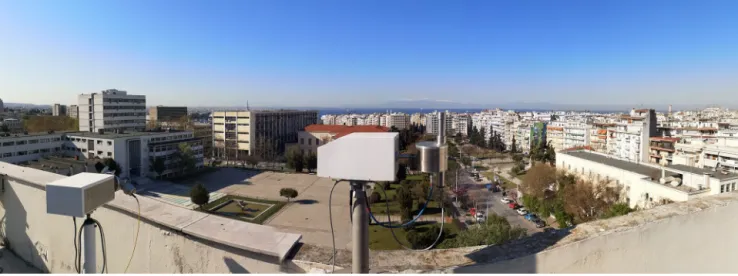
A 2D MAX-DOAS system (Phaethon) operates regularly on the rooftop (20 m above ground) of the Physics Depart- ment building of the Aristotle University of Thessaloniki (40.634^◦N, 22.956^◦E), about 60 m above sea level (a.s.l.).

The measurement site is located near the city center of Thessaloniki (Fig. 1). The prototype system was developed in 2006 at the Laboratory of Atmospheric Physics (LAP) (Kouremeti et al., 2008, 2013) and has been upgraded ever since for the retrieval of tropospheric NO₂VCDs (Drosoglou et al., 2017, 2018) and total ozone columns (Gkertsi et al., 2018). The current version of the system comprises a

single-channel ultra-low stray-light AvaSpec-ULS2048x64- EVO (f =75 mm) spectrometer by Avantes, the entrance optics, and a two-axis tracker. The spectrometer’s detector is a back-thinned Hamamatsu charge-coupled device (CCD) array of 2048 pixels with signal-to-noise ratio (SNR) 450:1 for a single measurement at full signal. The spectrometer covers the spectral range 280–539 nm and uses a 50 µm wide entrance slit. Mercury discharge lamp spectra were recorded to determine the instrument’s slit function, and the spectral resolution was found to be∼0.55 nm full width at half maximum (FWHM) at 436 nm. The spectrometer is positioned in- side a thermally isolated box, where the temperature is main- tained at+10^◦C using a thermoelectric Peltier system. The entrance optics are mounted on a two-axis tracker with two stepper motors controlling the azimuth viewing angle (0^◦≤ φ≤360^◦) and the elevation viewing angle (0^◦≤α≤90^◦) with pointing resolution of 0.125^◦, allowing both direct-sun and off-axis observations. A third motor rotates a filter wheel of eight positions with different optical components (diffuser, attenuation, and band-pass filters), used for the measurement of direct-sun and scattered radiation spectra and an opaque position for the measurement of the dark signal. The instrument operates automatically and is controlled by a custom- made software, developed at LAP. The entrance also comprises a telescope with a plano-convex lens that focuses the collected solar radiation onto one end of an optical fiber. The system’s field of view (FOV) was characterized using a dis- tant light source and was found∼1^◦. Simultaneous azimuth and elevation angle calibration are regularly performed by sighting the sun, so no horizon scans are necessary for the elevation angle calibration.

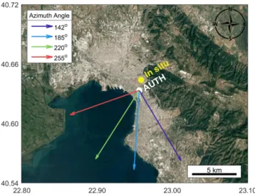
A routine MAX-DOAS measurement cycle starts by ori- enting the optics at a certain azimuth viewing direction followed by the measurement of scattered radiation spectra at the elevation angles: 90 (zenith), 30, 15, 12, 10, 8, 6, 5, 4, 3, 2, and 1^◦in this order. For this study, the system was configured to measure at four consecutive azimuth angles of 142, 185, 220, and 255^◦, illustrated in Fig. 2 with arrows of different colors. Based on the intensity of the measured spectra during an elevation scan at 142^◦azimuth, the viewing direction of the 1^◦elevation angle was found to be partly blocked by obstacles, such as trees and buildings in the campus. Thus, α=1^◦in this particular direction was excluded from the profiling analysis. In order to achieve high SNR values and to avoid saturated spectra, the number of scans of each individual measurement and the exposure time of the CCD are automatically adjusted by the operating software according to the received intensity by the detector. The integration time at each elevation angle is∼60 s, and a full measurement sequence for all azimuth directions lasts about 1 h.

(4)

Figure 1.The Phaethon MAX-DOAS system in the middle and a panoramic view (east–south–west) of the measurement site.

Figure 2. Location of the MAX-DOAS system (white dot) and the in situ NO₂ measurement site (yellow dot). The arrows in different colors represent the azimuth viewing directions, φ, of the MAX-DOAS observations (i.e., purple: 142^◦; blue: 185^◦; green: 220^◦; red: 255^◦). The base map is taken from

9538922,16768m/data=!3m1!1e3!5m1!1e4 (last access: 3 March 2022).

2.2 MAX-DOAS measurements and slant column retrieval settings

The primary retrieved product from the analysis of the measured MAX-DOAS spectra is the dSCD of several trace gases at different elevation angles. The dSCD of a trace gas at an elevation angle α(dSCD_α) can be calculated as the difference between the slant column density, i.e., its concentration integrated along the light path (SCD_α) and the SCD of a Fraunhofer reference spectrum (FRS), usually measured at

the zenith (SCD_ref):

dSCDα=SCDα−SCDref. (1)

The MAX-DOAS spectra that are used in this study have been recorded for 1 year (from May 2020 through May 2021), and a zenith spectrum is selected as the FRS in order to account for the Fraunhofer lines and the stratospheric contribution of the absorbers (Hönninger et al., 2004). Since the system is scheduled to perform both direct-sun and MAX-DOAS observations during the day, the zenith spectra of two consecutive elevation sequences may have a large time difference (duration of the first sequence plus the duration of two direct-sun measurements). So, in this study, the zenith spectrum of each sequence was selected as the FRS for the DOAS-based retrieval of the collision-induced oxygen complex (O₂–O₂ or O₄) and the trace gas dSCDs and not the average or the time-interpolated spectrum between the zenith spectra of the two consecutive sequences.

The dSCDs of O₄ and trace gases are derived from the recorded spectra by applying the DOAS technique (Platt and Stutz, 2008), while the measured spectra are analyzed using the QDOAS (version 3.2, September 2017) spectral fitting software suite developed by BIRA-IASB (https://uv-vis.

aeronomie.be/software/QDOAS/, last access: 5 March 2021) (Danckaert et al., 2013). The retrieval settings are based on results from the CINDI-2 campaign (http://www.tropomi.eu/

data-products/cindi-2/, last access: 5 March 2021) (e.g., Kre- her et al., 2020), the Quality Assurance for Essential Cli- mate Variables (QA4ECV) project (http://www.qa4ecv.eu/, last access: 5 March 2021), and the Network for Detec- tion of Atmospheric Composition Change (NDACC) pro- tocol for UV–VIS measurements (http://www.ndaccdemo.

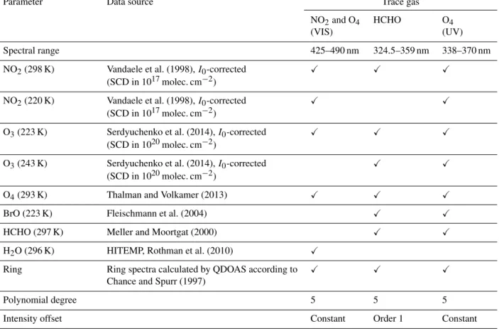
org/data/protocols/, last access: 5 March 2021). The spectral retrieval settings and the trace gas absorption cross sections that are included in the DOAS fit are listed in Ta- ble 1. The wavelength calibration of the measured spectra is

(5)

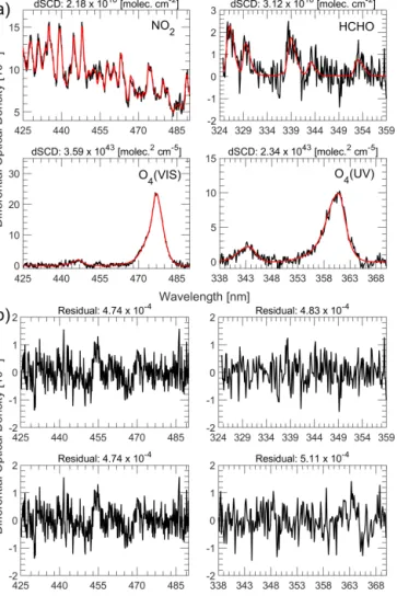
Figure 3.A typical example of the DOAS retrieval of NO₂, HCHO, O₄(VIS), and O₄(UV) dSCDs derived from a MAX-DOAS measurement on 9 July 2020 at 07:50 UTC (SZA=38.85^◦) at 3^◦viewing elevation angle. The DOAS fits are presented in the subpanels of panel(a). The black lines represent the measured spectra, and red lines are the fitted O₄and trace gas cross sections. The subpanels of panel(b)show the residual of the DOAS fits.

achieved by shifting and stretching them against a highly resolved solar reference spectrum (Chance and Kurucz, 2010).

Even though the spectrometer is operating in a temperature- controlled environment, small diurnal temperature variations may occur. Thus, dark spectra are measured after each elevation sequence for all of the exposure times that were used during the sequence. This procedure might be time- consuming, but it assures that the solar and dark spectra are measured at the same temperature. The dark spectra are then subtracted from the scattered radiation spectra prior to the DOAS analysis. Figure 3 shows a typical example of the DOAS analysis of a spectrum recorded on 9 July 2020 at 07:50 UTC at 3^◦elevation angle. During the whole period of study no apparent system-related issue or instrument degra- dation is observed.

2.3 Retrieval of the vertical profile

The retrieval of vertical profiles (extinction and concentration profiles for aerosols and trace gases, respectively) from MAX-DOAS measurements typically involves three major steps (Irie et al., 2011; Hendrick et al., 2014; Vlemmix et al., 2015b), independent of the retrieval approach. In the first step, the O₄ dSCDs and the trace gas dSCDs (in this case NO2and HCHO) are derived by applying the DOAS fitting technique to the measured spectra, as described in Sect. 2.2.

Next, the O4dSCDs retrieved for each elevation angle of the same sequence are used as input to the algorithm for the retrieval of the aerosol extinction vertical profile. In the end, the trace gas dSCDs are used as input to the algorithm for the retrieval of the trace gas vertical profile, along with the aerosol extinction profile, calculated in the previous step.

As mentioned already, the profiling algorithms that have been developed so far and are commonly used within the MAX-DOAS community are either based on the OEM or follow the parameterization approach. How the O₄and trace gas dSCDs are handled for the retrieval of the vertical profiles depends on each algorithm’s approach. However, the principal idea of both OEM and parameterized inversion algorithms is the same: a layered model atmosphere with defined parameters is assumed in a forward radiative transfer model (RTM), and it is used in order to simulate the O4and trace gas dSCDs, taking into account the viewing geometry, i.e., the solar zenith angle (SZA), the elevation angle, and the relative azimuth angle. The forward models and how the dSCDs are simulated are described in Beirle et al. (2019) for MAPA and in Friedrich et al. (2019) for MMF. The extinction and concentration vertical profiles are derived by invert- ing the forward model, i.e., by finding the model parameters, for which the difference between the simulated and the measured dSCDs is minimized, based on a cost function.

2.4 MMF

The Mexican MAX-DOAS Fit (MMF) v2020_04 (Friedrich et al., 2019) is an OEM-based profiling algorithm that relies on online RTM simulations using VLIDORT version 2.7 (Spurr, 2006) as forward model. The input parameters for each atmospheric layer are calculated from temperature and pressure profiles, the trace gas concentration in each layer, and the aerosol properties. The aerosol properties, which are the same for all layers, are the single-scattering albedo (SSA) and the asymmetry parameter (using the Henyey–Greenstein phase function, Henyey and Greenstein (1941), to calculate the phase function moments). Furthermore, the wavelength of the retrieval and the surface albedo need to be specified as additional input parameters. The retrieval algorithm comprises an aerosol extinction profile retrieval and a trace gas profile retrieval. The former constrains the aerosol extinction profile in the forward model of the trace gas retrieval. The inversion uses constrained damped least-square fitting with an

(6)

Table 1.DOAS fit settings for NO₂, HCHO, O₄(VIS), and O₄(UV).

Parameter Data source Trace gas

NO₂and O₄ HCHO O₄

(VIS) (UV)

Spectral range 425–490 nm 324.5–359 nm 338–370 nm

NO₂(298 K) Vandaele et al. (1998),I₀-corrected X X X

(SCD in 10¹⁷molec. cm⁻²)

NO₂(220 K) Vandaele et al. (1998),I₀-corrected X X

(SCD in 10¹⁷molec. cm⁻²)

O₃(223 K) Serdyuchenko et al. (2014),I₀-corrected X X X

(SCD in 10²⁰molec. cm⁻²)

O₃(243 K) Serdyuchenko et al. (2014),I₀-corrected X X

(SCD in 10²⁰molec. cm⁻²)

O₄(293 K) Thalman and Volkamer (2013) X X X

BrO (223 K) Fleischmann et al. (2004) X X

HCHO (297 K) Meller and Moortgat (2000) X X

H₂O (296 K) HITEMP, Rothman et al. (2010) X

Ring Ring spectra calculated by QDOAS according to X X X

Chance and Spurr (1997)

Polynomial degree 5 5 5

Intensity offset Constant Order 1 Constant

Wavelength calibration Based on a high-resolution solar reference spectrum (Chance and Kurucz, 2010)

optimal estimation regularization. In the used version, both the a priori and the covariance matrix are constructed. More details about the a priori settings and the input parameters can be found in Sect. 2.6. The retrieval algorithm provides the aerosol extinction profiles, trace gas partial column profiles, their integrated quantities, the corresponding noise and smoothing errors, the averaging kernel, the degrees of freedom, and a quality flag of the retrieval. The quality flagging system of MMF is based on the convergence of the algorithm, the root mean square of the difference between measured and simulated dSCDs, the reported degrees of freedom, and the stability of the retrieval.

2.5 MAPA

The Mainz Profile Algorithm (MAPA) v0.98 (Beirle et al., 2019) is a profiling algorithm developed by the Max Planck Institute for Chemistry (MPIC) that is based on a parameterization approach. MAPA does not rely on online RTM simulations, but its forward model is provided as pre-calculated differential air mass factor (dAMF) look-up tables (LUTs) at multiple wavelengths. These LUTs have been calculated offline by a full spherical RTM, McArtim (Deutschmann et al., 2011), following a backward Monte Carlo approach. Just like

MMF, MAPA is based on a two-step process in order to retrieve the aerosol and trace gas vertical profiles. It uses three main parameters to characterize the atmospheric profile: the column parameter, c(i.e., AOD for aerosols and VCD for trace gases); the layer height, h; and the shape parameter, s. Additionally, a fourth optional parameter can be included, the O₄scaling factor, which was initially introduced by Wag- ner et al. (2009) in order to achieve agreement between the measured dSCDs and the forward model simulations. Unlike MMF, MAPA is not based on the OEM, so no a priori as- sumption of the vertical profile is required. In some cases this can be an advantage since a priori information and constraints are usually difficult to estimate. MAPA also provides a detailed flagging algorithm that is based on thresholding techniques applied to different parameters, in order to evaluate whether the retrieved profile can be trusted. By default (and within this study), the flags are identical for the species retrieved in the UV and VIS spectral range. The flags that are defined in MAPA v0.98 are mainly based on the agreement between the measured and modeled dSCDs, the consistency of the derived Monte Carlo parameters, and the shape of the profile. More details about MAPA and its flagging algorithm can be found in Beirle et al. (2019).

(7)

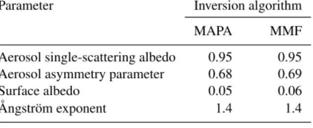
Table 2.The RTM settings that were used in MMF and MAPA for Thessaloniki.

Parameter Inversion algorithm

MAPA MMF

Aerosol single-scattering albedo 0.95 0.95 Aerosol asymmetry parameter 0.68 0.69

Surface albedo 0.05 0.06

Ångström exponent 1.4 1.4

2.6 Input parameters and settings

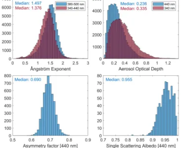
During MAPA calculations, depending on the aerosol or trace gas retrieval, a LUT corresponding to the central wavelength of the O₄or trace gas fitting window is selected (i.e., 360 nm for O₄ in the UV, 343 nm for HCHO, 460 nm for NO₂, and 477 nm for O₄in the VIS). These wavelengths are also used in the RTM simulations of MMF. For the calculation of the dAMF LUTs, MAPA’s radiative transfer simulations were performed with a typical fixed set of parameters for all wavelengths (Beirle et al., 2019), which can describe the majority of all potential measurement sites. MMF, on the other hand, relies on online RTM simulations, and so the aerosol and surface parameters can be adjusted to the most suitable values. In this study, the aerosol optical properties that are used as input for the simulations of MMF are based on 15 years of climatological data measured by a co-located CIMEL sun photometer. Figure 4 shows the frequency distribution of the Ångström exponent, AOD, asymmetry factor, and SSA in Thessaloniki, while their values that are used as input to each inversion algorithm are listed in Table 2. Dis- crepancies between MMF and MAPA due to small differences in these selected parameters are expected to be minor.

MMF requires a priori profile and covariance matrix information for the profile retrievals. The “a priori” term represents knowledge of the true state before the measurement is performed. However, the true shape of the trace gas vertical profiles at Thessaloniki is generally not known, while the true state of the aerosol profiles is known only in certain cases during the period of study. Thus, the retrieval is based on constructed exponentially decreasing a priori profiles with a scale height of 1 km, which are considered a reasonable estimate of the true profiles. Since no covariance matrix information is available, the covariance matrix is also constructed from the a priori profile. The AOD as well as the trace gas VCDs in Thessaloniki vary substantially through- out the year. In order to take into account the annual variability, we use the square of 50 % of the a priori on the diagonal elements of the covariance matrix for aerosols and 100 % for NO₂and HCHO. The loose constraint of the latter is due to the higher variability of the trace gas vertical columns over the course of the year. Both for aerosols and trace gases, the off-axis elements of the covariance matrix were constructed

by assuming a Gaussian function with a correlation length of 200 m, as described in Clémer et al. (2010). Additionally, based on empirical tests, the progress of the convergence is faster when using an a priori VCD or AOD below the true value for reasons that are not yet identified. Thus, the a priori AODs were set to 0.25 and 0.15 for the aerosol retrievals at 360 and 477 nm, respectively. For the trace gas retrievals we have used a priori VCDs of 4×10¹⁵and 6×10¹⁵molec. cm⁻² for NO₂and HCHO, respectively, based on data derived from the MAX-DOAS by applying the geometrical approximation (Hönninger et al., 2004) to the dSCDs measured at 30 and 15^◦ elevation angles. The LUTs used in MAPA cover the following ranges: 0–5 for the AOD, 0.02–5 km for the layer height, and 0.2–1.8 for the profile shape parameter (Beirle et al., 2019).

The temperature and pressure vertical profiles that are used as input in this study are identical for both MMF and MAPA.

We have used climatological profiles for Thessaloniki produced by MPIC that are based on∼16 years of re-analysis data from the European Centre for Medium-Range Weather Forecasts (ECMWF). The temperature and pressure profiles are interpolated to the day and time of each elevation sequence. We have also tried to use temperature and pressure profiles measured by radiosondes, launched on a daily basis at Thessaloniki Airport (∼13 km away from the measurement site), as input, but since no major effect is observed on the retrieved products, these results are not presented. Both algorithms are configured to export the retrieved vertical profiles to the same output grid ranging from the ground up to 4 km with 200 m vertical resolution.

As already mentioned, the recorded spectra are also analyzed by a central processing system in the frame of the FRM₄DOAS project. The analysis is carried out using default values of several parameters, which are reasonable for all potential measurement sites, while in this study we try to optimize the performance of MMF and MAPA in particular for Thessaloniki (see discussion above). In the FRM₄DOAS analysis a time-interpolated spectrum between the zenith spectra of two consecutive elevation sequences is used as the FRS for the dSCDs retrievals. Thus, the dSCDs that are used for the retrieval of the vertical profiles are slightly different than those used in the current study. The default FRM4DOAS settings include SSA of 0.92 and an asymmetry factor of 0.68. Yet, such small differences should have a negligible effect on the retrieved vertical profiles. The Ångström exponent is set to 1, and the same a priori aerosol extinction vertical profile (AOD of 0.18) is used for the retrievals in both the UV and VIS spectral ranges. The covariance matrices are constructed from the a priori profiles, but the square of 50 % of the a priori is used on the diagonal elements of the covariance matrices for all species. Currently, the partly blocked elevation angle of 1^◦at 142^◦azimuth (Sect. 2.1) is not excluded from the analysis. MAPA retrievals are performed using three different O₄scaling factors (i.e., 0.8, 1.0, and a variable scaling factor). In order to further investigate the effect

(8)

Figure 4.Frequency distribution of the Ångström exponent, AOD, asymmetry factor, and SSA measured by a CIMEL sun photometer in Thessaloniki for the period 2005–2021.

of the O₄ scaling factor (see Appendix A) in this study, we include an extra value of 0.9.

2.7 Ancillary data

This section briefly describes the supporting instruments that are used in this study for comparison and validation of MAX- DOAS-derived products. The ancillary data include measurements of a CIMEL sun photometer, a Brewer spectrophotometer, an aerosol lidar system, and an in situ NO₂monitoring station. Except for the in situ NO₂, all remote sensing instruments that are used in this study (i.e., the MAX- DOAS, CIMEL sun photometer, Brewer spectrophotometer, and lidar) are located at the same measurement site, about 60 m a.s.l. The effect of the different viewing geometries and the retrieval techniques that each system utilizes are discussed in the corresponding following sections.

2.7.1 CIMEL sun photometer

Since 2003 a sun–sky photometer (CIMEL) has provided spectral measurements of the AOD at Thessaloniki as part of the NASA’s Aerosol Robotic Network (AERONET) (https:

//aeronet.gsfc.nasa.gov/, last access: 5 March 2021). The CIMEL sun photometer is an automated, well-calibrated scanning filter radiometer specifically developed for the retrieval of the AOD at seven wavelengths (i.e., 340, 380, 440, 500, 670, 870, and 1020 nm) by using direct-sun observations. The technical specifications of the instrument are given in Holben et al. (1998). The instrument is calibrated regularly following the procedures and the guidelines of AERONET.

The AERONET database provides three distinct levels for data quality. Level 1.0 is defined as pre-screened data (i.e.,

no quality assurance criteria are applied). Version 3 (Sinyuk et al., 2020) of Level 1.5 represents near-real-time auto- matic cloud screened data, while Level 2.0 applies additional pre- and post-field calibrations. In this paper, we use the AERONET Level 1.5 data, since the Level 2.0 data for the period of study are not yet published. In order to compare with the AOD retrieved by the MAX-DOAS, the AODs at 360 and 477 nm have been calculated using the Ångström exponent between the standard spectral bands of the instrument.

2.7.2 Brewer spectrophotometer

The Brewer spectrophotometer with serial number 086 (B086) is a double monochromator that has performed spec- trally resolved measurements of the direct and global solar irradiance at Thessaloniki since 1993 (Bais et al., 1996; Foun- toulakis et al., 2016). The wavelength range of B086 is 290–

365 nm, and its spectral resolution is 0.55 nm at full width at half maximum (FWHM). The wavelength calibration is performed by scanning the emission lines of spectral discharge lamps, while maintenance of the absolute calibration is achieved by regularly scanning the spectral irradiance of a calibrated 1000 W quartz–halogen tungsten lamp (Garane et al., 2006).

Although the Brewer spectrophotometer’s initial purpose was the retrieval of total ozone columns, research activities have shown that the spectral AOD can be calculated from direct irradiance measurements by following two main ap- proaches: the first is based on the absolute calibration of the direct-sun spectra measured by the Brewer spectrophotometer (Kazadzis et al., 2005), while the second uses the Langley extrapolation method (relative calibration) (Gröbner and Meleti, 2004). In both cases the spectral AOD is calculated as the residual optical depth after subtracting the optical depths due to molecular scattering and the O₃and SO₂absorption from the total atmospheric optical depth (Kazadzis et al., 2007). Since 1997, the direct solar irradiance spectra measured by the Brewer spectrophotometer have been calibrated (Bais, 1997), so in this study we use the former approach (i.e., absolute calibration) for the retrieval of the spectral AOD. In order to compare with the AOD retrieved by the MAX-DOAS, the AOD at 477 nm is calculated using climatological monthly mean values of the extinction Ångström exponent derived from measurements of the CIMEL sun photometer in Thessaloniki. Details on the procedure of the Brewer spectrophotometer’s direct solar irradiance spectra absolute calibration as well as the spectral AOD retrieval methodology can be found in Bais (1997), Kazadzis et al.

(2005, 2007), and Fountoulakis et al. (2019).

2.7.3 Lidar

Thessaloniki has been a member station of the European Li- dar Aerosol Network (EARLINET, https://www.earlinet.org,

(9)

last access: 5 March 2021) since 2000, providing regu- lar aerosol profile measurements, following EARLINET’s schedule (Monday morning and Monday and Thursday evening), during extreme events and at satellite overpasses (e.g., AEOLUS, OMI).

THEssaloniki LIdar SYStem (THELISYS) is a multi- wavelength Raman/depolarization lidar system, which has been gradually upgraded regarding its operational wavelengths and the detection configuration. All the quality stan- dards, established within EARLINET, are followed in order to assure the high quality of the THELISYS products, which are publicly available in the EARLINET database (https:

//www.earlinet.org/index.php?id=125, last access: 5 March 2021). A detailed description of THELISYS technical specifications and algorithm can be found in Voudouri et al.

(2020).

The final products derived from the raw lidar data processing are the aerosol backscatter coefficient at 355, 532, and 1064 nm; the aerosol extinction coefficient at 355 and 532 nm; and the linear particle/volume depolarization ratio at 532 nm. During the day, the data acquisition is limited to the signals that arise from the elastic scattering of the laser beam by the air molecules and the atmospheric aerosol. The Klett–Fernald algorithm in backward integration mode is applied (Klett, 1981), and the backscatter coefficient profiles are produced. Constant a priori climatological values of the ratio between the extinction and the backscatter coefficient (lidar ratio) were assumed in this daytime method. Values of 60, 50, and 40 were used for 355, 532, and 1064 nm, respectively, given the atmospheric situations that occur over Thes- saloniki (Voudouri et al., 2020). The resulting uncertainties are discussed in depth by Böckmann et al. (2004) and can be as high as 50 % if there is no information about the actual lidar ratio, during extreme atmospheric conditions.

Another source of uncertainty during the lidar signal processing is the system’s overlap function, which determines the altitude, above which a profile contains trustworthy values. In our analysis, the correction is not available for the daytime retrievals. Thus, an overlap function from the previous nighttime measurement or a mean overlap profile is applied. The starting height is set to the full overlap height (approximately 0.6 km), assuming height-independent backscatter below 0.6 km, equal to the backscatter measured at this height, to account for both the incomplete overlap within the lidar profile and atmospheric variability in the lowermost tropospheric part. This overlap effect generally introduces uncertainties in the calculation of the columnar products (e.g., AOD). However, long-term comparisons (Siomos et al., 2018) have shown similar decreasing trends of the AOD at 355 nm between the EARLINET and the AERONET datasets (−23.2 % per decade and−22.3 % per decade, respectively).

The AODs at 355 nm measured by the lidar have also been compared with the Brewer spectrophotometer’s retrievals, showing a generally good correlation of 0.7 (Voudouri et al., 2017).

2.7.4 In situ

Near-surface concentrations of different air pollutants, including NO₂, NO, SO₂, CO, and O₃, are measured in Thes- saloniki by in situ instruments as part of the Network for Air Quality Monitoring of the Municipality of Thessaloniki. NO₂ is being monitored by chemiluminescence detectors that are mainly distributed around the city center. Most of the network stations are installed very close to the ground (sam- pling inlet at∼3 m) and are strongly affected by local traffic emissions. In this study, we use hourly mean (which is the highest available temporal resolution) in situ NO2 concentrations measured at the “Eftapyrgion” site (40.644^◦N, 22.957^◦E, 174 m a.s.l.), which is located in an urban back- ground area at a distance of∼1.2 km from the MAX-DOAS system to the north (Fig. 2). The in situ measurements, span- ning from May 2020 to March 2021, are used in order to validate the MAX-DOAS-derived NO₂near-surface concentrations. Even though this site is located opposite to the MAX- DOAS system’s azimuth viewing directions, it has been selected because the vertical and horizontal displacement of the two instruments is small, but also because it is the only site of the network almost unaffected by local traffic emissions and therefore can be considered more representative of the average NO2concentrations in the local boundary layer.

3 Results and discussion

In this section, we present results of the trace gas and aerosol quantities retrieved by the two inversion algorithms. We in- tercompare the dSCDs simulated by the forward models, the integrated columns (i.e., VCDs and AODs for trace gases and aerosols, respectively), the near-surface concentrations, and the seasonal mean vertical profiles between MMF and MAPA. Since MAPA is based on a parameterization approach, no information about averaging kernels is provided;

hence, results on averaging kernels are presented only for MMF.

The MAX-DOAS system operates at a site where the northern viewing directions are blocked by buildings of the campus and the city, so the system is configured to perform sequences of elevation scans at azimuth directions in the southern sector, as illustrated in Fig. 2. As a result, scattered radiation spectra may be measured during the day at azimuths close to the solar azimuth angle. In such cases, RTM simulations might face difficulties in properly calculating the dAMF due to increased aerosol forward scattering, usually leading to underestimation of the true dAMF. For small scattering angles the uncertainties caused by the incorrect description of the phase function can also become important, and the results for such viewing geometries should be treated with caution. Therefore, the elevation sequences measured at azimuth angles relative to the sun of less than 5^◦are excluded from the analysis. In addition, the elevation sequences, for

(10)

which the retrieved AOD from the MAX-DOAS inversion algorithms is greater than 1.5, are filtered out, since such high aerosol loads are unrealistic for Thessaloniki (Fig. 4). Nega- tive columns can occur in the trace gas retrievals of MAPA within the Monte Carlo ensemble, and they are by default not removed, but this is not possible for MMF retrievals since, in its current version, MMF operates in logarithmic state vec- tor space. For NO₂, no valid negative columns are retrieved, but for HCHO, MAPA reports negative columns for∼8.5 % of the valid data. In order to compare meaningful results between the two algorithms, the negative columns are removed from the initial dataset.

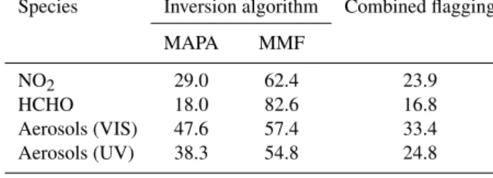
The individual flagging schemes of MMF and MAPA have been discussed elsewhere. Based on synthetic data, Frieß et al. (2019) reported that the quality flagging criteria of MAPA might be too strict, since a large fraction of data were flagged as invalid, even though the algorithm successfully removed almost all outliers. In our study, MAPA flags a larger fraction of data as invalid, compared to MMF, for all the retrieved species. The percentage of the valid data flagged by MAPA and MMF (individually and combined) is presented in Table 3. Since in MAPA retrievals no a priori constraints are used, more strict flagging needs to be applied for retrieved dSCDs that are characterized by large uncertainties (e.g., due to larger fit error or the effects of clouds). Espe- cially for HCHO, the apparent worse performance of MAPA could be explained by the lower SNR in the UV, along with the higher HCHO profile height compared to NO2(see discussion in Sect. 3.5) and the decreasing sensitivity towards higher altitudes. The retrieval results are sensitive to the va- lidity flagging approach, which is further investigated in the next section. No cloud filtering is applied to the data prior to the profiling analysis. Neither MMF nor MAPA include a direct cloud flagging system. However, some flags that are included in the flagging algorithms of MMF and MAPA are sensitive to clouds. Hence, in order to achieve retrievals of high quality and to ensure that the MAX-DOAS measurements performed under broken cloud conditions are filtered out, an elevation sequence is considered valid as long as it is flagged as valid by both MMF and MAPA. This is the default flagging scheme for NO₂, HCHO, and AOD at 477 nm, and all the results shown in the next sections follow this flagging approach unless stated otherwise. For AOD at 360 nm the flags reported by MAPA are considered default, since this approach performs better when comparing the MAX-DOAS results with other reference instruments (Sect. 4), although the reason for this behavior has not yet been identified. Also, since the issue for selecting the optimum O₄ scaling factor remains unresolved (Beirle et al., 2019; Wagner et al., 2019, 2021), we let MAPA determine an optimum O₄scaling factor (variable) for each elevation sequence, and this option is selected as the default for the retrievals.

It should be noted that in the following sections an orthogonal distance regression (ODR or bivariate least-squares) has been used instead of an ordinary linear regression (OLR or

Table 3.The fraction of the data ( %) that are flagged as valid by MMF and MAPA (individually and combined) for each species.

Species Inversion algorithm Combined flagging

MAPA MMF

NO₂ 29.0 62.4 23.9

HCHO 18.0 82.6 16.8

Aerosols (VIS) 47.6 57.4 33.4

Aerosols (UV) 38.3 54.8 24.8

standard least-squares) for the comparison of the retrieved products derived by MMF and MAPA, in order to equally treat the two algorithms since none of them depend on the other. The discrepancies in the regression slopes and in- tercepts arising in the OLR when comparing independent variables, and the appropriateness of ODR, are discussed in Cantrell (2008). The ODR results are also sensitive to the assumed errors of the two variables. The uncertainty contained in the MAX-DOAS measurements may be difficult to assess, but, since both MMF and MAPA retrievals are based on the same input data, the associated errors are assumed the same and equal to the mean error provided by MMF and MAPA for each data point.

3.1 Simulated dSCDs

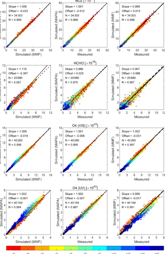
In this section we evaluate the performance of the forward models of MMF and MAPA by intercomparing the simulated trace gas dSCDs of the four species for the entire period. Also, we assess their ability to successfully simulate the slant column densities under different atmospheric (pollution and meteorological) conditions and viewing geometries by comparing the modeled with the measured dSCDs (Fig. 5). Each row corresponds to a different trace gas, with the left column presenting the intercomparison results of the modeled dSCDs, while the middle and right columns show the comparison results between the measured dSCDs and the dSCDs simulated by MAPA and MMF, respectively. The data points are colored by the elevation angle, and hotter colors represent dSCDs close to the horizon. A generally better performance of both algorithms is observed for the species retrieved in the VIS range compared to those retrieved in the UV. The modeled slant columns agree well, with Pearson’s correlation coefficients and slopes close to unity (R=0.999, slope=1.008 for NO₂andR=0.998, slope=1.006 for O₄ VIS). Additionally, the simulated dSCDs are in good agreement with the measured dSCDs, which is a good indicator for successful profile retrievals. In the case of O₄(UV), even though the slope and correlation coefficient are similar to O₄ (VIS), a larger scatter is evident, while for HCHO larger deviations from unity in the slopes and correlation coefficients are observed, especially at higher elevation angles. This can probably be explained by the increased noise in the UV spec-

(11)

tra compared to the VIS range and also due to the fact that at higher elevation angles the measured differential optical densities are very low, reaching the spectrometer’s detection limit. For aerosols in both spectral ranges, discrepancies between the simulated dSCDs of MMF and MAPA may arise due to the variable O₄scaling factor that is included in MAPA retrievals. This could also be the main driver of the positive bias for low elevation angles that is found in MMF’s O₄dSCDs (especially in the UV), while the results of MAPA are less affected.

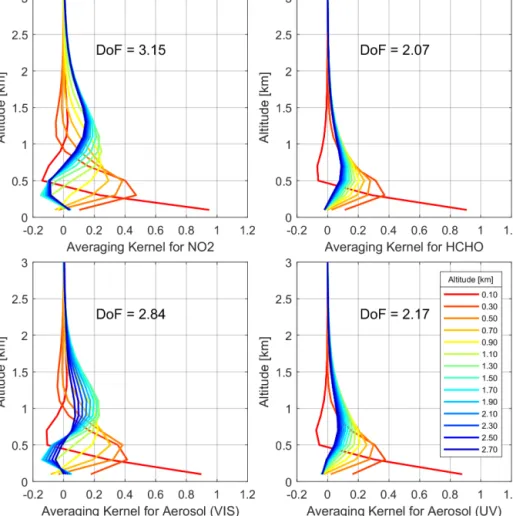
3.2 Averaging kernels

The averaging kernels (AVKs) of a profile retrieval describe the sensitivity of the retrieved state to the true atmospheric state for each altitude layer. The degrees of freedom (DoFs) are mathematically derived as the trace (or sum of the diagonal elements) of the AVK matrix and quantify the number of independent pieces of information gained from the measurements compared to the a priori knowledge (Rodgers, 2000).

Both the AVKs and the DoFs can be used to characterize the quality of the retrieved profile. Since only OEM-based inversion algorithms are capable of providing AVKs, the results shown here are derived only by MMF. Figure 6 shows a typical example of the calculated AVKs for each of the retrieved species, including their corresponding DoFs. The median DoFs retrieved by MMF are 3.13±0.32 for NO2, 2.22±0.34 for HCHO, 2.73±0.28 for aerosols in the VIS, and 2.02±0.32 for aerosols in the UV. The averaging kernels illustrate that MAX-DOAS measurements are typically less sensitive for altitudes greater than ∼2 km, as a result of the viewing geometry, and thus, altitudes greater than 3 km are not presented here. That means that the MAX- DOAS measurements under these viewing geometries and with the a priori profiles and covariance matrices used in this study (Sect. 2.6) are adequate for retrieving the extinction and concentration profiles only up to the lowermost ∼1.5–

2 km of the atmosphere with the highest sensitivity closer to the ground. Also, since the photon path increases with wavelength, the MAX-DOAS technique shows higher sensitivity for the species retrieved in the VIS range than in the UV.

3.3 Integrated columns

In the past, the trace gas VCDs measured by our MAX- DOAS systems have been derived by dividing the measured dSCDs, only at two elevation angles, 30 and 15^◦, or the mean of the two, with appropriate dAMFs. The dAMFs have been calculated either following the geometrical approximation approach or by deploying RTM simulations taking into account the viewing geometry, the aerosol optical properties, and the instrument’s viewing direction relative to the sun (Drosoglou et al., 2017). However, in both cases, the actual trace gas profile has not been taken into consideration, intro- ducing, possibly, an additional uncertainty to the measured

VCD. This is the first time during the Phaethon’s operation that the whole elevation sequence is used in order to retrieve the tropospheric VCDs more accurately. The comparison of the NO₂and HCHO VCDs that are derived from the integration of the vertical profiles with the VCDs that are calculated using the geometrical approximation can be found in the Ap- pendix B.

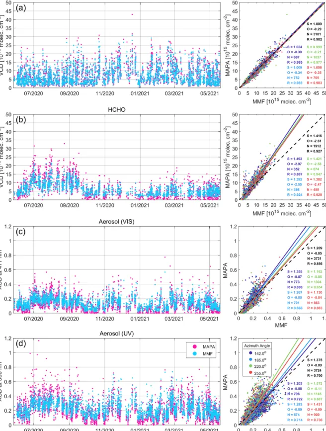
In Fig. 7 the time series of the integrated columns of all retrieved species (i.e., AODs for aerosols and VCDs for trace gases) are presented, as well as comparisons between MMF and MAPA. The statistics of the comparisons, i.e., slope (S), offset (O), number of points (N), and Pearson’s correlation coefficient (R), are shown in different colors for each azimuth viewing direction. The text in black color represents the consolidated statistics for all azimuth directions. No clear azimuth dependence of the retrieved columns is observed for the trace gases. However, for aerosols, especially in the UV, significant differences in the regression slopes appear for the different azimuths. It should be noted that in these comparisons a variable O₄ scaling factor has been used for the MAPA retrievals, and since no scaling factor has been applied to the MMF retrievals, differences in the AODs between the two algorithms are expected. The number of elevation sequences at 220^◦azimuth is always larger compared to the other azimuth directions, because the instrument was configured to record spectra only at this particular direction for approximately 1 month in the beginning of its operation.

The comparison shows that the NO2VCDs derived by MMF and MAPA are in very good agreement, with slopes and correlation coefficients close to unity (ranges: 0.999≤S≤ 1.024 and 0.977≤R≤0.985). Similar results were obtained for all azimuth directions withS=1.009 andR=0.982. In the case of HCHO, despite the good correlation (R=0.927), notable deviations from unity in the slope are observed for all azimuth directions. MAPA systematically reports larger VCDs than MMF for higher HCHO concentrations, while the opposite behavior is observed for low HCHO loads, indicating that further investigation is required. This behavior could be explained by the increased spectral noise in the UV that leads to discrepancies between the HCHO dSCDs simulated by the forward models of MMF and MAPA (see discussion in Sect. 3.1) and due to an invariant a priori profile during the year. The sensitivity of the MAX-DOAS decreases with altitude and it is very limited at altitudes above

∼2.5 km for the species measured in the VIS spectral range or even lower (∼1.5 km) for the species in the UV (Fig. 6).

For NO₂, this is generally not a problem since the total column is dominated by the concentration in the lower layers of the troposphere (see also discussion in Sect. 3.5). How- ever, HCHO can be vertically extended at higher altitudes, where the sensitivity of the MAX-DOAS is low. In the case of HCHO, MMF is more prone to result in the a priori profile, while MAPA retrievals become more unstable. Thus, the vertical profiles of MAPA are expected to have greater variability. Concerning aerosols, the comparison of the retrieved

(12)

Figure 5.Intercomparison of the dSCDs simulated by MMF and MAPA (left column) and comparison of the dSCDs simulated by MAPA (center column) and MMF (right column) against the measured dSCDs. The elevation angles are denoted by different colors (see scale at the bottom).

(13)

Figure 6.A typical example of the retrieved averaging kernels for different altitudes of each species. Hotter colors correspond to altitudes closer to the ground.

AODs reveals better agreement at 477 nm (R=0.856) than at 360 nm (R=0.700), with larger scatter and more outliers compared to the trace gas VCDs. As already mentioned, this is mainly attributed to the O₄ scaling factors that are used in MAPA retrievals. More details about the effect of the O₄ scaling factor on the retrieved AODs and the trace gas VCDs can be found in Appendix A.

3.4 Surface concentrations

The surface concentration is defined as the trace gas amount at ground level. However, the profile parameterization used within MAPA allows for the retrieval of lifted trace gas layers for a shape parameter greater than 1, which leads to a value of zero for the concentration at the surface. For these cases, the comparison with in situ measurements or surface concentrations retrieved by an OEM-based algorithm will be low-biased. Thus, in the following sections, the term “surface concentration” will refer to the mean “near-surface concentration”, i.e., the average concentration below 200 m for both MMF and MAPA, rather than the concentration directly at the ground. Figure 8 shows the time series of the near-

surface NO₂and HCHO concentrations derived by MMF and MAPA and the corresponding scatter plots. The comparisons of the surface values are similar to the comparisons of the tropospheric VCDs (shown in Fig. 7) with slope=1.118,R= 0.919 for NO₂and slope=1.295,R=0.855 for HCHO, but more outliers are present. In the case of HCHO, the surface concentrations derived for the 142^◦azimuth direction show larger differences compared to the other directions, while this is not clear for NO2. These discrepancies are possibly related to the fact that for this azimuth, the elevation angle of 1^◦was not included in the analysis (see Sect. 2.1), which may have influenced the retrieved surface concentrations.

3.5 Seasonal mean vertical profiles

Figure 9 shows the seasonal mean NO₂, HCHO, and aerosol extinction vertical profiles at Thessaloniki retrieved by MMF (cyan) and MAPA (magenta) during the 12 months considered in this study. Each row represents the vertical profiles of a specific species, and each column corresponds to a different season. The shaded areas represent the standard deviation around the mean for each layer, and they illustrate

(14)

Figure 7.Time series and scatter plots of the integrated columns for all species retrieved by MMF and MAPA (panelarefers to NO₂,bto HCHO,cto aerosols in the visible range, anddto aerosols in the UV). The parameters of the orthogonal distance regression, i.e., slope (S), offset (O), number of points (N), and Pearson’s correlation coefficient (R), are shown in different colors for each azimuth viewing direction.

The text in black color represents the consolidated statistics for all azimuth directions. The dashed black line represents the 1:1 line.

(15)

Figure 8.Time series and scatter plots of the near-surface concentrations of NO₂(a)and HCHO(b)derived by MMF and MAPA. The parameters of the orthogonal distance regressions are presented as in Fig. 7.

the seasonal variability of the vertical profiles. For NO2both algorithms report profiles that are decreasing with altitude for all seasons. Compared to MAPA, MMF reports slightly lower NO₂concentrations below 1 km (yet within the range of variability) and slightly higher above 1 km. For all seasons, the variability of MMF’s profiles between 1 and 2 km is larger, probably due to the increased contribution of the a priori profile under certain conditions (e.g., high aerosol load or fog close to the ground), where the sensitivity of the MAX-DOAS is lower. However, the seasonal mean profiles of both algorithms indicate that most of the NO₂content lies within the first∼500 m. NO₂originates mainly from direct, local emissions close to the ground (e.g., road transport emissions). Additionally, its lifetime in the PBL is short, typically a few hours depending on the season (e.g., Beirle et al., 2011; Liu et al., 2016), and as a result, higher NO2amounts are expected at lower altitudes in the troposphere. Both algorithms retrieve higher concentrations close to the surface during the cold period, which can be mainly attributed to enhanced NO₂emissions near the ground (e.g., from domestic heating sources) and to reduced photolysis rates due to weaker solar radiation.

An opposite seasonal variation is observed for HCHO, with higher concentrations reported by both algorithms during summer (consistent with the VCDs, shown in Fig. 7). The profile shapes of MMF and MAPA agree reasonably well.

In summer, the larger retrieved concentrations are probably due to the increased emissions of VOCs, whose oxidation produces HCHO. According to Zyrichidou et al. (2019), biogenic emissions are expected to peak during summer, while the anthropogenic emissions do not show a clear seasonal variation in Thessaloniki. Therefore, the observed HCHO seasonality is mainly attributed to the enhanced biogenic emissions from vegetation in summer. VOCs are generally well mixed and have longer life times (Chan et al., 2019), hence, larger HCHO amounts are expected at higher altitudes during the warm season. MMF’s profiles peak at a slightly higher altitude (∼800 m) than MAPA’s (∼500 m) and decrease with a slightly higher rate and less variability for altitudes above 1 km. However, such differences, especially at higher altitudes, are to some extent expected, since the sensitivity of the MAX-DOAS decreases rapidly with altitude for the species that are measured in the UV (Fig. 6). This means that concentrations at high altitudes are strongly constrained by the a priori profile in the retrievals of MMF. Also, parameterized algorithms (such as MAPA) have the tendency of becoming unstable when the sensitivity is low (Frieß et al., 2019).

For aerosols, the largest differences in the vertical profiles of MMF and MAPA are found in the VIS range and especially in summer and autumn. MMF yields more structured aerosol extinction profiles for altitudes between 1 and

(16)

2 km, while MAPA reports smoother, exponentially decreasing profiles. Such differences are not found in the UV retrievals during summer and autumn. It should be noted that larger discrepancies among different inversion algorithms for the species retrieved in the VIS compared to the UV have also been reported in other studies (e.g., Frieß et al., 2019; Tir- pitz et al., 2021). At higher altitudes, both algorithms report greater aerosol concentrations in summer than the winter, in both the UV and VIS. Similar results were found for Thessa- loniki by Siomos et al. (2018) using seasonal mean vertical profiles measured by a lidar system. In contrast, near the surface, aerosol concentrations are highest in winter and lowest in summer. This pattern can be mainly attributed to the shal- lower PBL in Thessaloniki during winter and autumn that shrinks to ∼1 km (Georgoulias et al., 2009; Siomos et al., 2018) due to the weaker solar radiation and lower air tem- peratures. In the UV during winter, MAPA retrieves larger aerosol concentrations close to the ground, which decrease more rapidly with altitude than MMF. However, as already discussed for HCHO, the sensitivity of the MAX-DOAS in the UV is very limited at higher altitudes, and the profiles of MMF are driven towards the a priori profile. Another con- tributing factor for the differences in the aerosol extinction profiles between the two algorithms might be the variable O₄ scaling factor that is used in MAPA retrievals, while no scaling factor is applied in MMF. The effect of the O₄ scaling factor on the AOD is presented in the Appendix A.

4 Validation

In this section we present the validation results of the products retrieved by the MAX-DOAS profile analysis against ancillary data measured by other reference co-located instruments. Vertical profiles of the aerosol extinction measured by a co-located lidar system are used to validate the aerosol vertical profiles retrieved by the MAX-DOAS, while the AODs in the UV and VIS range are compared with those measured by a sun photometer and a spectrophotometer. The NO₂ near-surface concentrations are compared with in situ surface measurements, but since no other sources of HCHO data are available, the MAX-DOAS-derived vertical profiles, columns, or surface concentrations cannot be validated.

4.1 Aerosol extinction profiles

The AOD values at 477 and 360 nm retrieved by the MAX-DOAS are compared with the AOD measured by the co-located CIMEL sun photometer and the Brewer spectrophotometer. Quasi-simultaneous (within ±15 min) measurements were found, and the AODs at 477 and 360 nm were calculated using the Ångström exponent between 380 and 500 nm and the AOD at these wavelengths derived by the CIMEL sun photometer. Since the Brewer spectrophotometer’s wavelength range spans up to 365 nm, climatological

monthly mean Ångström exponent values, calculated from the CIMEL data, have been used to extrapolate the AOD to 477 nm. Figure 10 shows the time series of all AOD data at 477 and 360 nm (not just the quasi-simultaneous) retrieved by the three systems. The CIMEL sun photometer was not operating for approximately 4 months during the summer of 2020 due to a delay in its scheduled annual maintenance and calibration. AOD data derived by the Brewer spectrophotometer are available until January 2021.

Since MMF and MAPA rely on their own individual flagging schemes in order to ensure that the retrieved products are of high quality, we investigate the effect of applying different flagging schemes to the data, which are listed in Ta- ble 4.

Scheme nos. 1 and 2 correspond to the default own flagging algorithms of MMF and MAPA, scheme no. 4 is expected to provide data of maximum quality since data are designated as valid by both algorithms, while scheme no. 3 rejects the error-flagged data but treats the warnings raised by MMF or MAPA as valid data. Figure 11 shows the comparison between the common AOD data derived by the CIMEL sun photometer, Brewer spectrophotometer, and the MAX- DOAS at 360 and 477 nm. Each column of the figure corresponds to a different flagging scheme as described in Ta- ble 4. Figure 12 graphically presents the statistics of the linear regressions (i.e., slope, offset, number of points, and Pearson’s correlation coefficient) between the reference instruments and the MAX-DOAS. The panels (a)–(d) correspond to different flagging schemes, as Fig. 11.

The comparison results of the MAX-DOAS against the CIMEL sun photometer are slightly different than those with the Brewer spectrophotometer. This can probably be explained by the fact that only a few collocated measurements are available and in different periods for the two reference instruments (Fig. 10). In the case of the AOD at 477 nm most of the outliers are filtered out when the flagging scheme no. 4 is applied, and the best agreement is observed between the reference instruments and the MAX-DOAS, for both MMF and MAPA, with similar correlation coefficients (0.79 for the CIMEL sun photometer and 0.81 for the Brewer spectrophotometer). Compared to the CIMEL sun photometer, MAPA seems to perform slightly better than MMF when each algorithm considers its own flagging, with correlation coefficients of 0.70 and 0.50, respectively (MAPA for scheme no. 2 and MMF for scheme no. 1). However, compared to the Brewer spectrophotometer, both algorithms show very similar correlation coefficients (0.78 and 0.77). Swapping the flags between MMF and MAPA leads to worse agreement and more outliers. The results of scheme no. 3 indicate that some of the warning-flagged data are of lower quality and should be treated with caution.

In the case of the AOD at 360 nm, the effect of the flagging schemes is different. Here, most of the outliers are eliminated, and the best overall agreement is achieved for scheme no. 2 (i.e., when MAPA’s individual flagging algo-

(17)

Figure 9.The seasonal mean vertical profiles of NO₂, HCHO, and aerosol extinction in the VIS and UV retrieved by MMF and MAPA. Each row (1–4) represents the vertical profiles of different species along the four seasons (columns 1–4). The shaded areas represent the standard deviation around the mean for each layer, and they illustrate the seasonal variability of the profiles.

rithm is applied). This behavior is observed for both MMF and MAPA, indicating that the flagging algorithm of MAPA performs better than that of MMF in the UV. The correlation coefficients with the CIMEL sun photometer data are 0.72 for MAPA and 0.70 for MMF, and with the Brewer

spectrophotometer data they are 0.72 for MAPA and 0.78 for MMF. The flagging scheme no. 4 removes even more data (as expected) but does not improve the comparisons.

The effect of the warning-flagged data (scheme no. 3) is more apparent in the case of the UV, and the results sug-

Retrieval of tropospheric aerosol, NO2, and HCHO vertical profiles from MAX-DOAS observations over Thessaloniki, Greece: intercomparison and validation of two inversion algorithms

Retrieval of tropospheric aerosol, NO 2 , and HCHO vertical profiles from MAX-DOAS observations over Thessaloniki, Greece:

intercomparison and validation of two inversion algorithms

Retrieval of tropospheric aerosol, NO ₂ , and HCHO vertical profiles from MAX-DOAS observations over Thessaloniki, Greece: