The Belgian Federal Planning Bureau (FPB) is a public body under the Prime Minister and the Minister of Economy. -03 The usage tables for imported goods and for trade margins - An integrated approach to the preparation of the Belgian 1995 tables. In this working paper, we describe the new quarterly model for the Federal Planning Bureau.
More precisely, we present the specification and estimation results of the model's main behavioral equations, and provide an overview of the overall accounting structure. Since 1994, the Federal Planning Bureau has used the annual version of the econometric model MODTRIM1 as the central tool for drawing up its short-term macroeconomic forecasts2. On that occasion, the opportunity was taken to reassess all of the model's behavioral equations.
The simultaneous response of the full model to exogenous shocks is investigated through various technical simulations and scenario analyses. These forecasts serve as the background for the preparation of the federal government's revenue and expenditure budget.
II Model specification and estimation results
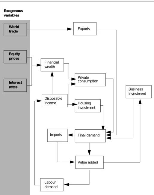
- The main characteristics of the model
- Households
- Firms
- Foreign trade
- Prices and wages
- The institutional sectors’ accounts
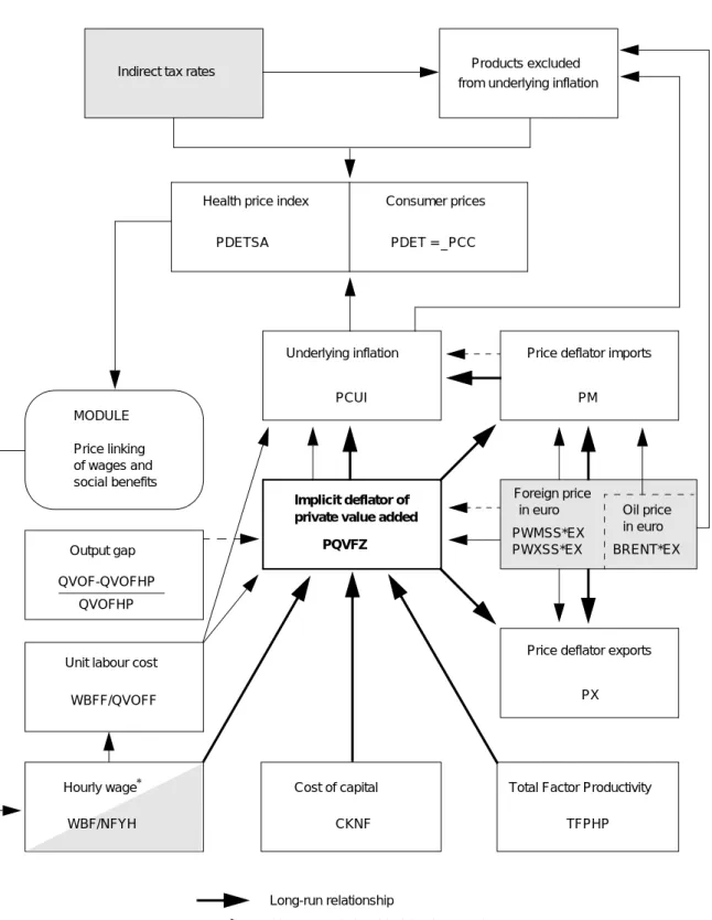
The deflator of private added value derived from the Cobb-Douglas production function plays a central role in the price formation mechanisms of the model. A glossary of the names for the various variables used in the behavioral equations is provided in Appendix II. Publications describing such models only give a snapshot of the state of the model at a certain moment.
The development of unemployment is an important explanatory factor for short-term consumer spending. Labor demand is only endogenous in the private sector wage earner model. The demand for capital1 is also derived from the Cobb-Douglas function, however taking into account medium-term fluctuations in the share of capital depending on the profitability of private sector value added.
The cost of capital is defined as a function of the long-term real interest rate, the corporate investment deflator, and the rate of capital depreciation. The coefficient of the lagged endogenous variable is negative, reflecting the jagged profile of the series. First-order serial correlation is still present despite the introduction of a lagged endogenous variable on the right-hand side of the equation.
The implicit private value added deflator derived from the Cobb-Douglas production function plays a central role in the price formation mechanisms of the model. This implies that the growth rate of this deflator may be slightly different from the growth rate of the implied deflator generated by the equation mentioned in the previous section1. In the long run, exporting firms are assumed to set prices as a weighted average of international export prices (expressed in euros) and (long-run value of) domestic value-added prices, the coefficient of the latter reflecting the price scale. the creativity they have.
The first three products are not taken into account for the calculation of the health index. Nevertheless, it is also influenced by the simultaneous evolution of the implicit deflator of private value added and of unit labor costs and by the previous growth of import prices. Among the nine excluded products, only the modeling of the two energy prices (fuel for vehicles and energy products for heating and lighting) is presented below.
In the tables below, the codes in parentheses at the beginning of the various items refer to ESA 1995. The codes in parentheses at the end of the various items refer to the model variable names.
III Model simulations
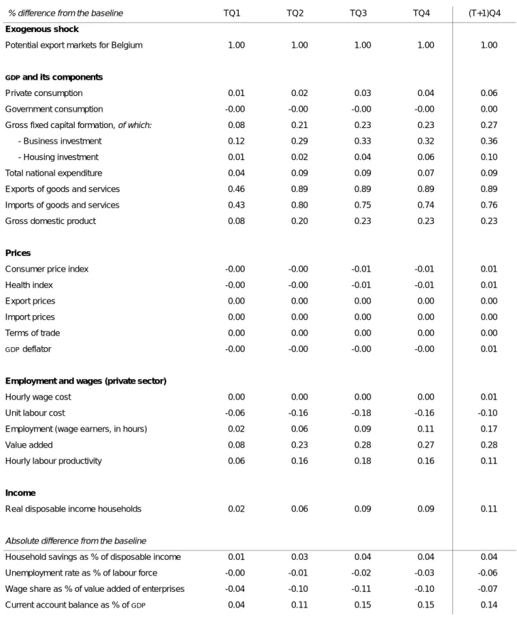
Technical simulations
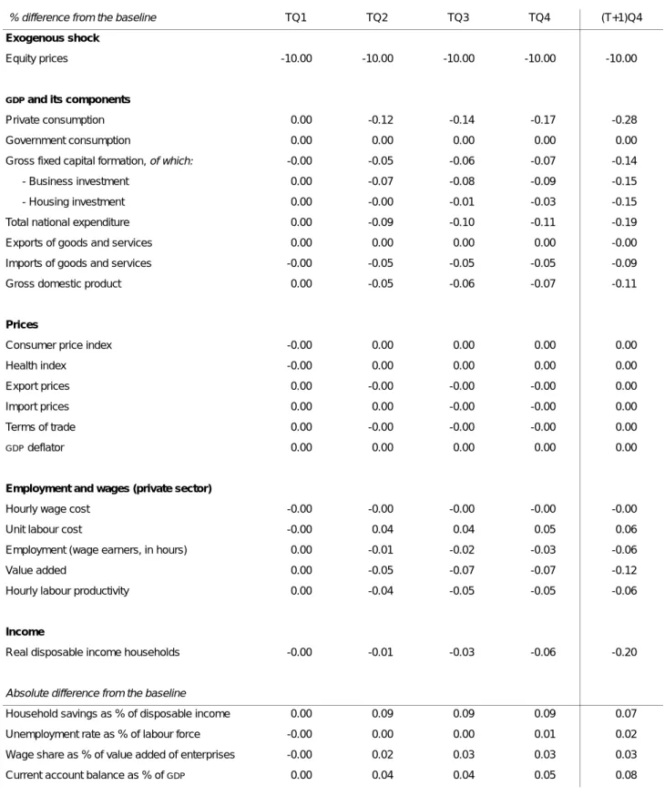
Due to the high two-quarter cumulative short-term elasticity and the high coefficient of the error correction term, adjustment to the new long-term level (+0.89%) was already achieved during the second quarter. This increase in external demand is satisfied by an increase in production, which causes extra business investment (+0.32% at the end of the first year). This naturally reinforces the wealth effect described above, so that private consumption decreases by 0.28% at the end of the second year.
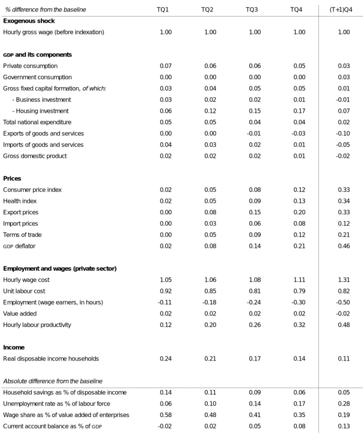
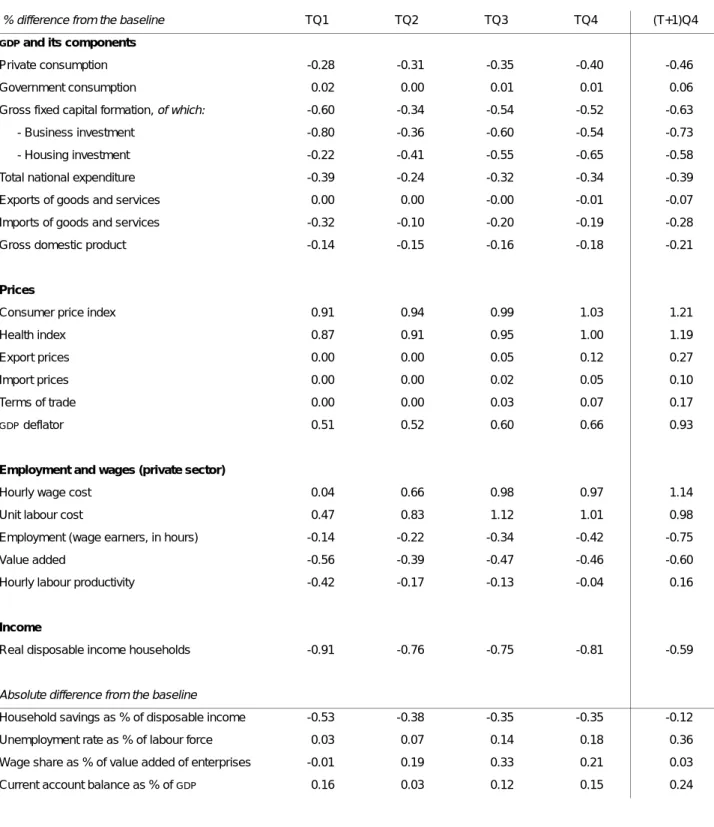
Gross hourly wages (excluding indexation) are exogenous in the current version of the model. In this scenario, an additional wage increase of 1% is considered during the first quarter of the simulation period. The result is that after an initial increase, consumption expenditure gradually returns to its baseline level (it is only 0.05% above the baseline at the end of the first year).
As prices rise slowly, due to higher labor costs, exports begin to decline at the end of the first year due to a weakening in price competitiveness. The increase in real disposable income is less than half of its initial level at the end of the simulation period, because the acceleration in inflation (CPI . ends 0.33% above the baseline) has a negative impact on real estate income and weighs job destruction on wage income. This represents approximately 251 million euros during the first quarter and 268 million euros at the end of the simulation period.
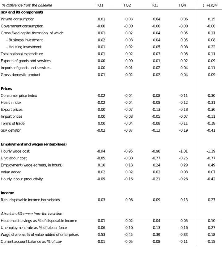
Employment in the private sector increases by 0.10% in the first quarter and by 0.29% at the end of the first year. Since prices are quite sticky, the slowdown is only gradual (-0.11% for the CPI and -0.18% for export prices at the end of the first year). In the first quarter after the shock, the impact on employment is quite limited, as most of the fall in value added is initially offset by lower productivity (productivity cycle).
During the first two years after the shock, private consumption is less affected than households' real disposable income, as the lower savings rate absorbs part of the shock. Exports are not affected during the first year after the shock and only marginally during the second year, as higher domestic labor costs are passed on to export prices, weakening cost competitiveness with the rest of the world. Deflated by the private sector value added deflator (from a producer's point of view). . below the baseline in Q4), followed by a very limited additional impact during the second year (-0.21% in (T+1)Q4).
Scenarios
As employment continues to rise, and as indexation gradually reduces purchasing power losses, real disposable income somewhat exceeds the baseline during the second year. As a result, private consumption is slightly higher than in the reference scenario at the end of the simulation period (0.01%). Domestic prices rise steadily during the simulation period, which means that GDP associated with stabilizing losses in the terms of trade.
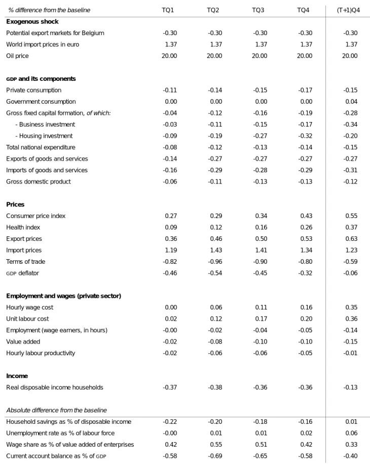
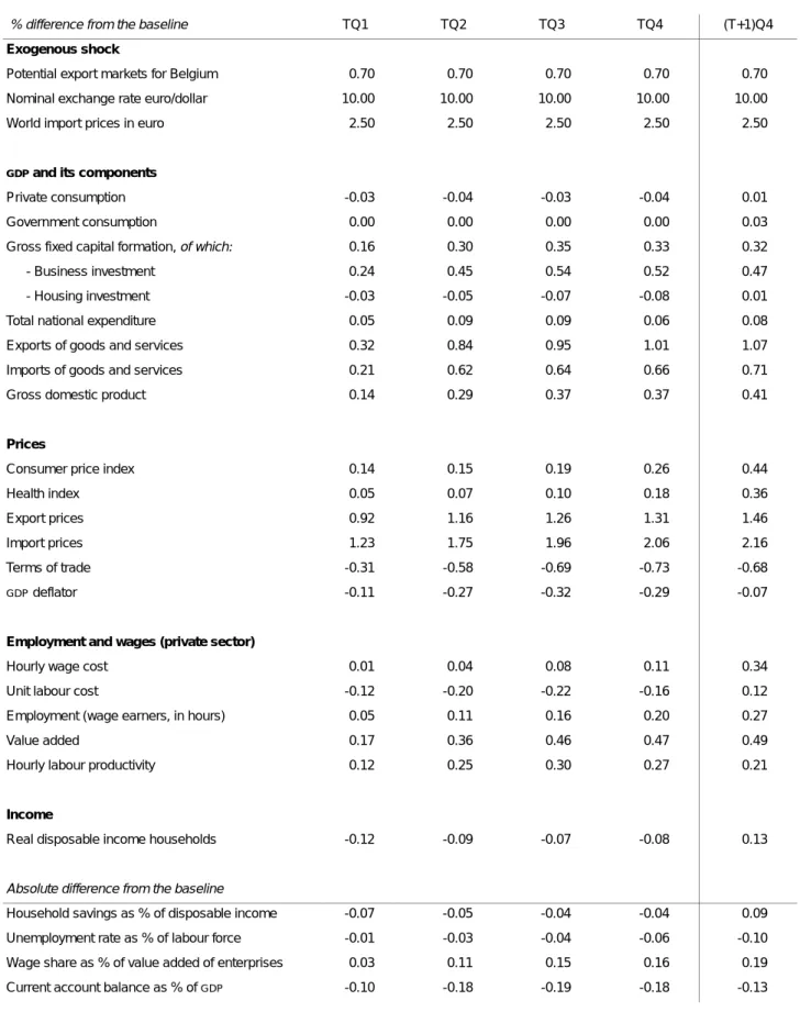
Finally, the impact on the current account balance is still negative at the end of the second year (-0.13%), as higher net exports in volume have not yet fully offset the trade loss. In this scenario, we analyze the effects of an increase in the crude oil price, which raises the Brent oil price expressed in dollars 20% above its level in the baseline scenario during the entire simulation period. For a net oil importing country like Belgium, the oil price shock works through the economy as a negative shock on the terms of trade, leading to a loss of real disposable income of the entire economy.
Nevertheless, the deterioration of the terms of trade exceeds the growth of the domestic demand deflator during the entire simulation period, which means that the GDP deflator has not yet returned to its baseline level after two years. As wages and social benefits are linked to the development of the health index and the latter does not take into account higher vehicle fuel prices, the difference in growth between the consumer price index and the health index (around 0.18%) accounts for any permanent loss of household purchasing power. The modifications of other exogenous variables below are based on CPB (2002) and Dalsgaard et al.
This measure is more or less identical to the inverse of the wage share, given in the table below. During the entire simulation period, private consumption is less affected than households' real disposable income, as the lower savings rate absorbs part of the shock. While housing investment returns somewhat to its baseline level during the second year after the shock, business investment continues to decline.
Changes in relative prices are considered to have no impact on exports and imports due to the specific nature of the shock (oil prices). Four quarters after the oil price shock, GDP at constant prices is 0.13% lower than in the base scenario. During the second year after the shock, this difference remains virtually unchanged1 (-0.12% after eight quarters).
The quarterly data base
Glossary of variable names
Summary accounts of the four institutional sectors
The households’ summary account
The corporations’ summary account
The general government summary account
The external transactions account of the nation
Regression statistics