General and selective reductions in employer social security contributions in the 2002 vintage of HERMES - A revision of WP 8-01. BFPB's activities are mainly focused on macroeconomic forecasting, analysis and assessment of policies in the economic, social and environmental fields.
Abstract
I Heterogeneous labour in HERMES
Three categories of endogenous labour
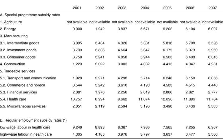
Defining special-programme employment
The size of the reductions in employer contributions to social security schemes and wage subsidies provided by 'Plan Activa' depends on the age and unemployment benefit status of the recruited workers. It is important that the reductions in employer contributions to social security schemes become less generous, as the 'Dienstenbanen'/'Emplois-service' with 100% exemption is replaced by 'Plan Activa'.

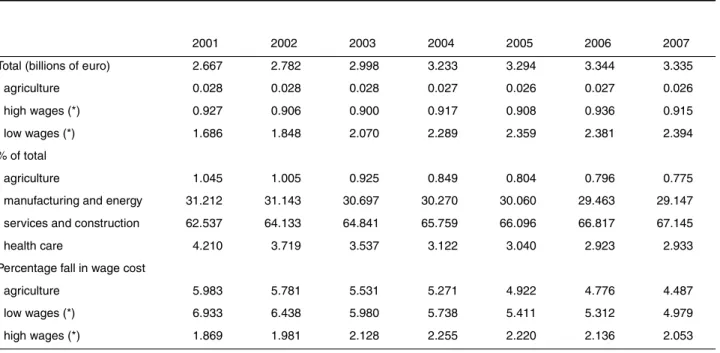
Labour-specific wage cost rates
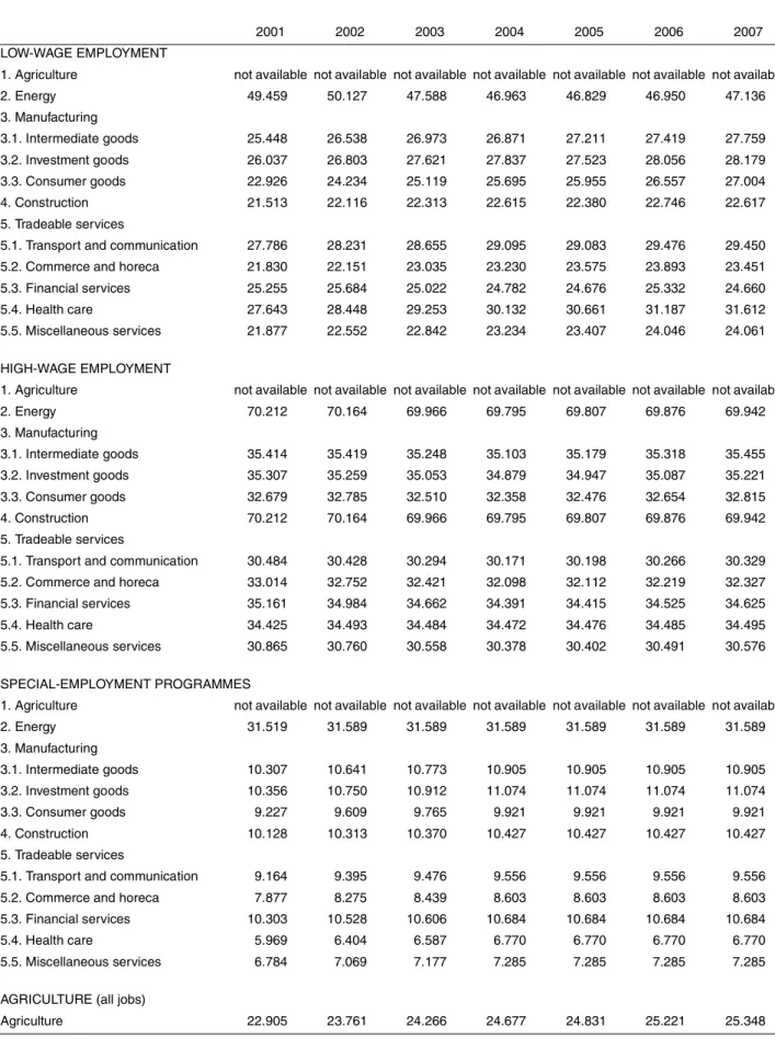
Other factors can influence the level of employer social security contributions: (1) changes in the composition of the workforce because blue-collar and white-collar workers face different statutory contributions; (2) the size of the company, (3) changes in extralegal, sector-specific contributions (Masure, 2001). Agriculture not available not available not available not available not available not available not available.
II Modelling substitution in the Belgian labour market
- Modelling heterogeneous labour in HERMES
- Translog-based substitution
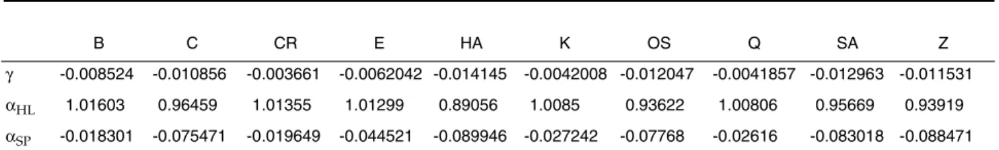
- Calibration
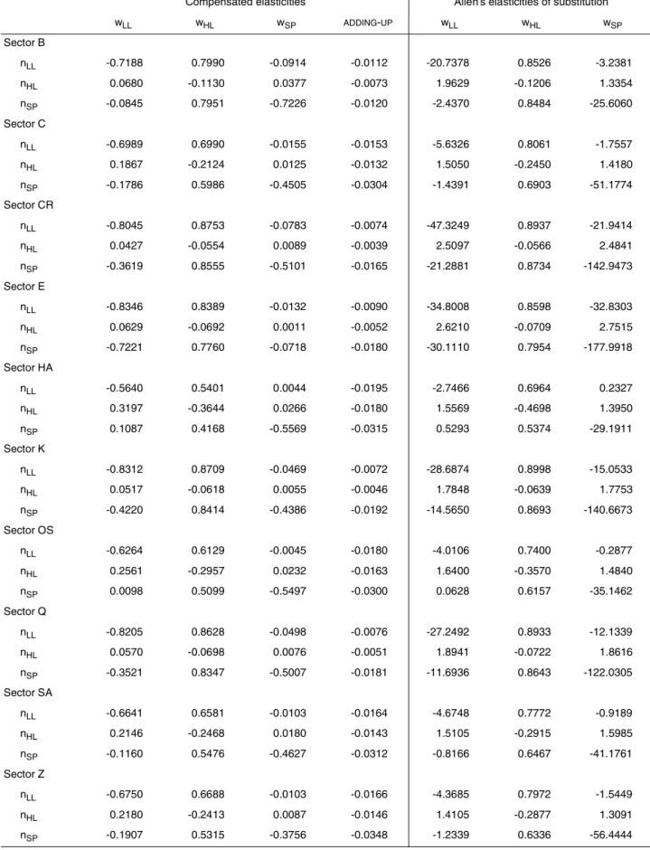
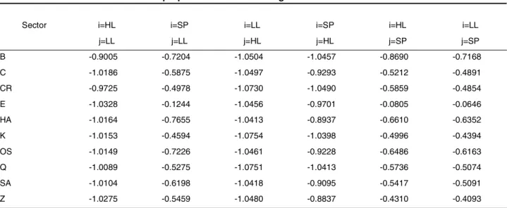
- Labour demand: Compensated price elasticities and Allen’s elasticities of substitution
- The empirical literature on substitution in the labour market
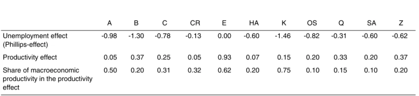
Allen elasticity of substitution indicates substitution between LL and HL and between HL and SP. They operate with elasticities of substitution of up to 1.1 (internationally competitive market sector), 2.0 (internationally non-competitive market sector) and 1.5 (non-market sector).
III Two baselines
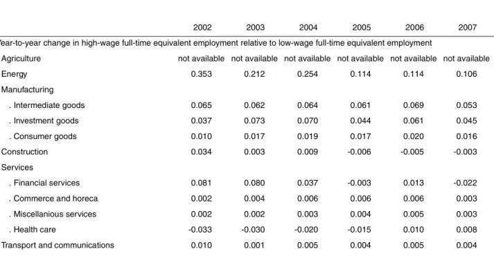
Substitution in the 2002-2007 baseline forecast with wage benchmarking
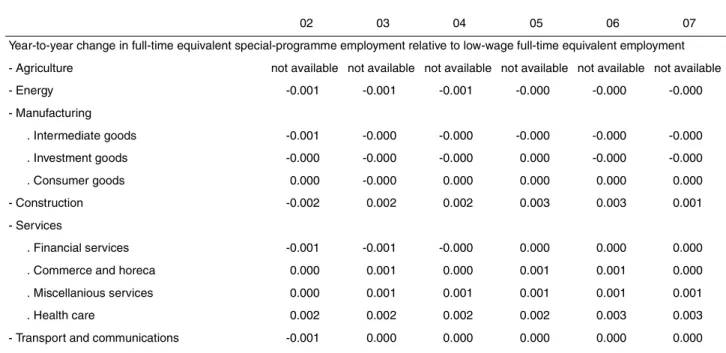
Year-over-year change in the equivalent cost of the high full-time salary compared to the equivalent cost of the low full-time salary. Year-over-year change in full-time equivalent employment in special programs relative to full-time equivalent employment at low wages - Agriculture not available not available not available not available not available.
The 2002-2007 baseline forecast with free wages
- Macro-economic feedback
- Caveat: A proper free-wage baseline?
- Caveat: Differences in wage-regime specific baselines?
These social security contribution rates likely underestimate the true rates prevailing in a self-employment scheme. On the one hand, the prior reduction in a free salary sentence should be smaller for two reasons. With gross wage rates higher in the free wage scheme and due to the structural measure's bias in favor of low wages, the prior reduction per employed to be smaller in size.
On the other hand, the free wage regime's gross wage bill is likely to be higher despite lower employment. The free-wage and wage-benchmark baselines differ in income and employment levels. This matters because the same increase in output requires a greater increase in employment in a wage-benchmark regime than in a free-wage regime.
In Table 11,
IV Additional reductions in employer social-security contributions
Limitations and caveats
- Normal and special employment
- Two sets of policy simulations
- Caveat: Interpreting substitution in the labour market
- Caveat: wage cost and employment
- Caveat: total, wage-earning and self-employed labour
- Caveat: other considerations
- Caveat: comparison with previous HERMES policy simulations
The first set assumes the same government-sanctioned gross wage benchmark as in the baseline medium-term forecast. In addition, it is assumed that the self-employed and salaried workers receive the same average wage cost rate. Whether this matters in policy simulations depends on how self-employment is modeled in those sectors (i.e. all sectors except CR, OS and SA).
If the self-employed labor force is modeled as a trend, the self-employed labor force is unaffected relative to the baseline and the net jobs created are entirely attributable to wage labor. If the self-employed labor force is modeled as a ratio of employment, as in the case of the commercial sector (HA), the net jobs created are distributed between self-employed and wage labor. However, labor demand in financial services (CR), miscellaneous services (OS), and health care (SA) is modeled in terms of wage employment, and total employment is determined by adding self-employed workers to wage workers.
If self-employment is modeled as a trend (as in SA), self-employment is unaffected relative to the baseline, and wage-earning labor is the only source of net job creation. If self-employment is modeled as a ratio of employment as in the case of CR and OS, additional wage-earning employment tends to have a leverage effect and additional self-employment is created, increasing total employment.
Reductions in employer social-security contributions in the case of wage benchmarking
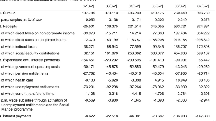
- Employment and public finances
- Sectoral output
- Aggregate demand
- Winners and losers: firms, households, the government and the economy nation-wide
The reason is that the low-wage measure destroys high-paying jobs and thus income from income tax and social security contributions. The effectiveness of labor cost reduction policies, especially low wage measures, is probably overestimated due to the weight of self-employed work in net job creation. This phenomenon is particularly strong in the case of the low wage measure due to strong job creation in HA and OS (see more).
The effect of employment on disposable income is particularly strong in the case of the low-wage measure, but the overall effect on the wage bill is softened by the substitution of high-wage work for low-wage work. Overall, the high wage measure is slightly stronger than the low wage measure in raising private consumption (0.027% vs. 0.021%). Note that the low wage measure elicits the largest changes in the profitability and cost competitiveness of wages.
Judging by GDP and employment, the measure of low wages is the most beneficial for the entire country. If the criterion were company profitability, companies would also prefer low wages.
Reductions in employer social-security contributions in the case of free gross wage setting
Whatever the wage regime, consumer goods, manufacturing and agriculture benefit more from the low-wage measure than other sectors. However, due to the low-wage measure, the financial sector expands relatively more in a free-wage setting than in a wage-benchmark regime, probably because the Phillips effect on wages in the financial sector is relatively small . In contrast, capital goods manufacturing suffers from the low-wage measure if wages are exempted, probably because of the relatively strong Phillips effect on wages in that sector.
Apart from weaker effects in a free-wage regime, sector output reacts qualitatively in the same way as the high-wage target in the two wage regimes. The smaller decrease in labor costs per unit of output accounts for the smaller increase in GDP if wage setting is free, especially when the low wage measure is implemented. In terms of employment and business welfare, the low wage measure is the most beneficial policy.
However, when judged by consumption, there is not much difference between the high-wage measure and the low-wage measure. The high-wage measure is still the most expensive policy in terms of net cost per job, but the drop in government surplus it generates is barely different from the one generated by the low-wage measure.
V Conclusions
VI References
1999), "Forfaitaire" verlaging van werkgeversbijdragen en gelijkschakeling tussen beroepscategorieën, [Ad capita vermindering van werkgeversbijdragen voor sociale zekerheid en geleidelijke afschaffing van discriminatie tussen functiecategorieën], Federaal Planbureau, ADDG, 6138.
VII Appendum 1: Conditional employment programmes: an overview
Measures existing prior to 2002
For continued continuous employment after the expiry of the employment contract, the company may be entitled to a permanent reduction of the employer's social security contributions in the amount of 10% of the gross salary, if the former employee is employed on the basis of a permanent employment contract. indefinite duration and if this means a net increase in the number of employees in the company.
Measures existing as from 2002
VIII Appendum 2: Medium-term policy simulation results (t+6)
Wage benchmark
2] c:/usr/simulations/update-sim/norm-LL.var [3] c:/usr/simulations/update-sim/norm-HL.var [4] c:/usr/simulations/update-sim /norm-LLHL.var [5] c:/usr/simulations/update-sim/norm-SP.var. absolutne razlike glede na izhodišče – milijoni evrov). 1] c:/usr/simulations/update-sim/norm-base.var [2] c:/usr/simulations/update-sim/norm-LL.var [3] c:/usr/simulations/update-sim /norm-HL.var [4] c:/usr/simulations/update-sim/norm-LLHL.var [5] c:/usr/simulations/update-sim/norm-SP.var. 1] c:/usr/simulations/update-sim/norm-base.var [2] c:/usr/simulations/update-sim/norm-LL.var [3] c:/usr/simulations/update-sim /norm-HL.var [4] c:/usr/simulations/update-sim/norm-LLHL.var [5] c:/usr/simulations/update-sim/norm-SP.var (/) Stop hier.
Free wages
1] c:/usr/simulations/update-sim/free-base.var [2] c:/usr/simulations/update-sim/free-LL.var [3] c:/usr/simulations/update-sim /free-HL.var [4] c:/usr/simulations/update-sim/free-LLHL.var [5] c:/usr/simulations/update-sim/free-SP.var. 1] c:/usr/simulations/update-sim/free-base.var [2] c:/usr/simulations/update-sim/free-LL.var [3] c:/usr/simulations/update-sim /free-HL.var [4] c:/usr/simulations/update-sim/free-LLHL.var [5] c:/usr/simulations/update-sim/free-SP.var (/) Stop hier.
IX Appendum 3: Transitional and medium- term simulation results in an economy
- The low-wage measure (scenario ‘LL’)
- The high-wage measure (scenario ‘HL’)
- The low-wage cum high-wage measure (scenario ‘LLHL’)
- The special-programme measure (scenario ‘SP’)
1] c:/usr/simulations/update-sim/norm-basis.var [2] c:/usr/simulations/update-sim/norm-LL.var (-) Differences. absolute differences with baseline - millions of euros). 1] c:/usr/simulations/update-sim/norm-basis.var [2] c:/usr/simulations/update-sim/norm-LL.var (/) Growth rates. 1] c:/usr/simulations/update-sim/norm-basis.var [2] c:/usr/simulations/update-sim/norm-HL.var (-) Differences. absolute differences with baseline - millions of euros).
1] c:/usr/simulations/update-sim/norm-basis.var [2] c:/usr/simulations/update-sim/norm-HL.var (/) Groeipercentages. 1] c:/usr/simulations/update-sim/norm-base.var [2] c:/usr/simulations/update-sim/norm-LLHL.var (-) Verschillen. absolute verschillen met de basis - miljoen euro). 1] c:/usr/simulations/update-sim/norm-base.var [2] c:/usr/simulations/update-sim/norm-LLHL.var (/) Groeipercentages.
1] c:/usr/simulations/update-sim/norm-base.var [2] c:/usr/simulations/update-sim/norm-SP.var. absolute verschillen met de basis - miljoen euro). 1] c:/usr/simulations/update-sim/norm-base.var [2] c:/usr/simulations/update-sim/norm-SP.var (/) Groeipercentages.
X Appendum 4: Transitional and medium- term simulation results in an economy
The low-wage cost measure (scenario ‘LL’)
1] c:/usr/simulaties/update-sim/vrij-basis.var [2] c:/usr/simulaties/update-sim/vrij-LL.var (-) Differences. absolute differences with baseline - millions of euro). 1] c:/usr/simulaties/update-sim/vrij-basis.var [2] c:/usr/simulaties/update-sim/vrij-LL.var (/) Growth Rates. 1] c:/usr/simulaties/update-sim/vrij-basis.var [2] c:/usr/simulaties/update-sim/vrij-HL.var. absolute differences with baseline - millions of euro).
1] c:/usr/simulations/update-sim/free-base.var [2] c:/usr/simulations/update-sim/free-HL.var (/) Groeipercentages. 1] c:/usr/simulations/update-sim/free-base.var [2] c:/usr/simulations/update-sim/free-LLHL.var. absolute verschillen met de basis - miljoen euro). 1] c:/usr/simulations/update-sim/free-base.var [2] c:/usr/simulations/update-sim/free-LLHL.var (/) Groeipercentages.
1] c:/usr/simulations/update-sim/free-base.var [2] c:/usr/simulations/update-sim/free-SP.var. absolute verschillen met baseline - miljoenen euro's).