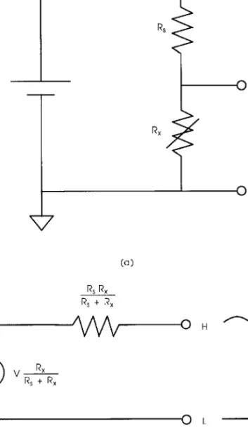
If terminal L is at ground potential (grounded supply in Figure 80.1a), the signal is single-ended and grounded. In Figure 80.5, the transfer function for each noise source is the same as that of the signal vd.
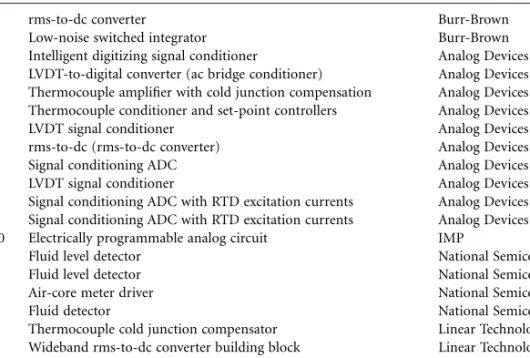
Special-Purpose Signal Conditioners
Horenstein, Microelectronic Circuits and Devices, 2nd ed., Englewood Cliffs, NJ: Prentice-Hall, 1996, is an introductory electronics textbook for electrical or computer engineering students. Dostál, Operational Amplifiers, 2nd ed., Oxford, UK: Butterworth-Heinemann, 1993, provides a good combination of theory and practical design ideas.
Introduction
Continuous data filters are further divided into passive or active filters, depending on the type of elements used in their implementation. Depending on the type of signal processed by such a filter, a distinction can be made between an analog sampled data filter and a digital filter.
Filter Classification
Filters can be classified based on the input, output and internal operating signals. In a sampled data filter, on the other hand, the signal is sampled and processed at discrete instants of time.
The Filter Approximation Problem
The zeros of Y(s) given by s = s0i which are equivalent to the zeros of Ha(s) are called the transmission zeros of the filter. Stability constrains the poles of Ha(s) to lie in the left half of the s-plane excluding the jW axis, i.e. Re{s¥i} < 0. Usually the amplitudes of the allowed ripples for the magnitude response are given in decibels.
Therefore, this approximation is also FIGURE 82.2 The quadratic magnitude function of an analog filter can have ripple in the passband and stopband. Filter order ie. N, is then selected so that the brake band specifications are met. Wp = frequency at the edge of the passband (for a specified waviness of the passband) Ws = frequency at the edge of the stopband (for a specified bottom of the stopband) N = order of the polynomial.

Design Examples for Passive and Active Filters
The element values in Table 82.3 are numbered from the source end in the same way as in Figure 82.4. The simplest first-order (N = 1) active filter is the first-order passive filter of Figure 82.3 with the addition of a unity gain-follower amplifier. The most commonly used two-pole active filter circuits are the Sallen and Key low-pass resonator, the multiple feedback bandpass, and the state-variable implementation as shown in Figure 82.7a, b, and c.
The transfer function and design equations for the Sallen and Key circuit in Figure 82.7a are. The multiple feedback circuit of Figure 82.7b is a minimum component count, two-pole (or one-pole pair), bandpass filter circuit with user-definable gain. For convenience, Figure 82.7c equates several of the resistors and identifies others with subscripts that relate to their function in the circuit.

Discrete-Time Filters
The zeros of the polynomial X(z) given by z = z¥i are called the poles of H(z) and are commonly referred to as the natural frequencies of the filter. The condition for the stability of the filter is expressed by the restriction that all the poles of H(z) must lie inside the unit circle, i.e. The zeros of Y(z) given by z = z0t, which are equivalent to the zeros of H(z), are called the transmission zeros of the filter.
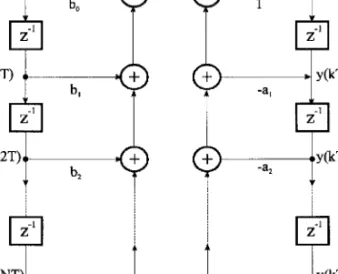
Clearly, at these frequencies the output of the filter is zero for any finite input. Note that the element values for the multipliers are obtained directly from the numerator and denominator coefficients of the transfer function. Physically, the input numbers are samples of a continuous signal, and real-time digital filtering involves computing the iteration of Equation 82.43 for each incoming new input sample.
Digital Filter Design Process
FIR Filter Design
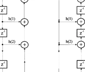
The purpose of FIR filter design is to determine N ± 1 coefficients given by. 82.50) so that the transfer function H(ejwT) approximates a desired frequency characteristic. Note that because Equation 82.47 is also in the form of a convolution summation, the impulse response of an FIR filter is given by . These quantities are depicted in Figure 82.12 for a prototype low-pass filter. dp and ds characterize the allowable errors in the passband and in stopband, respectively.
82.55), where hd(kT) is the corresponding impulse response sequence that can be expressed as Hd(ejwT). 82.56). Some commonly used windows are Bartlett (triangular), Hanning, Hamming, Blackmann, etc., definitions of which can be found in Reference 15. The most commonly used method for designing FIR filters with optimal magnitude is the Parks–McClellan algorithm.
IIR Filter Design
The next step involves the derivation of a corresponding analog transfer function for the analog prototype. As can be seen from Equation 82.66, the analog frequency domain (imaginary axis) maps onto the digital frequency domain (unit circle) nonlinearly. Convert the critical digital frequencies (e.g., wp and ws for low-pass filters) to the corresponding analog frequencies in the s-domain using the relationship given by Equation 82.67.
As explained earlier, these poles lie equally spaced in the s-plane on a circle of radius Wc. 82.70) Using the bilinear transformation. gives a digital transfer function. Filters realized by directly using the structure defined by Equation 82.44 are called direct IIR filters. Two less sensitive structures can be obtained by partial fractional expansion or by factoring the right-hand side of Eq. 82.46 in terms of real rational functions of order 1 and 2.
Wave Digital Filters
82.73), where the transfer function for the kth building block is 82.74) Note that this form is obtained by factoring Equation 82.45 in second-order sections. In order to fully establish an equivalence with classical circuits, the interconnections are also simulated by so-called wave adapters. The most important of these interconnections are series and parallel connections, which are simulated by series and parallel adapters, respectively.
In the next step, the electrical elements of the LC filter are replaced by its digital realization using Figure 82.15.

Anti-Aliasing and Smoothing Filters
It is generally desirable to reduce all aliasable frequency components (at frequencies greater than half the sampling rate) to less than the LSB of the ADC in use. If it is possible that the aliasable input can have an amplitude as large as the full input signal range of the ADC, then it is necessary to attenuate it with the full 2N range of the converter. The amount of attenuation required can be significantly reduced if there is knowledge of the input frequency spectrum.
Additional considerations in antialiasing the system are noise and distortion introduced by the filter that is supposed to eliminate aliasable inputs. It is possible to have a perfectly clean input signal which, when passed through a prefilter, has noise and harmonic distortion components in the frequency range and of sufficient amplitude to be within a few LSBs of the ADC. It is necessary that both noise and distortion components in the output of the anti-alias filter should also be kept within a LBS of the ADC to ensure system accuracy.
Switched Capacitor Filters
While an anti-aliasing filter on the input avoids unwanted errors that would result from undersampling the input, a smoothing filter on the output reconstructs a continuous-time output from the discrete-time signal applied to its input. Since each bit of an ADC represents a factor of 2 of those adjacent to it, and 20 log(2) = 6 dB, the minimum attenuation required to reduce a full-scale input to less than an LSB is . For example, some sensors, due to their electrical or mechanical frequency response, may not be able to produce a full-scale signal at or above the Nyquist frequency of the system and therefore "full-scale" protection is not required.
In many applications, even for 16-bit converters that would require 96 dB of anti-alias protection at worst, 50 to 60 dB is sufficient. The ADC cannot distinguish between an actual signal present in the input data and a noise or distortion component generated by the prefilter.
Adaptive Filters
Depending on the application, the variations in the coefficients are performed according to an optimization criterion and the adjustment is performed at a rate up to the sampling rate of the system. Some of the most commonly used adaptive algorithms are LMS (least mean square), RLS (recursive least squares) and frequency domain, also known as block algorithm. A number of adaptive algorithms and structures can be found in the literature that meet different optimization criteria in different application areas.
They are applied before the sampling is performed to prevent aliasing in the sampled version of the continuous time signal. Equiripple: Characteristic of a frequency response function whose magnitude exhibits equal maxima and minima in the passband. High-pass filter: A filter that passes all frequencies above its cutoff frequency and stops all frequencies below it.

Spectrum Analysis and Correlation Ronney B. Panerai
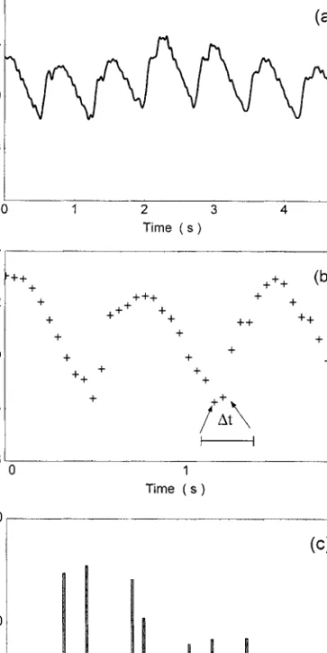
Since ck is complex (Equation 83.6b), a more physically meaningful interpretation of the spectrum is given by the amplitude and phase spectrum, defined as . The main point in the amplitude spectrum corresponds to the frequency of the cardiac cycle in Figure 83.1a. 83.13) where Sk is usually called the autospectra of xn.6 Equation 83.13 shows that it is possible to estimate the power spectrum from a previous estimate of the autocorrelation function.
The periodicity of the ACF reflects the quasi-periodic pattern of the intracranial pressure signal (Figure 83.1a). Instead of a single harmonic at the frequency of the original sinusoid, the power spectrum estimated by the FFT will have power at other harmonics, as indicated by the spectrum in Figure 83.5c. It is possible to show that when the observation period T tends to infinity, equation 83.8 gives an unbiased estimate of the power spectrum.
83.22) which shows that the reliability of power spectrum estimates can be improved by increasing m. However, this effect is compensated for in Equation 83.24, and in this case the mean value effect is the addition of a constant term:.