ON THE COMPONENTS OF SPACES OF CURVES ON THE 2-SPHERE WITH GEODESIC CURVATURE IN A PRESCRIBED INTERVAL
NICOLAU C. SALDANHA AND PEDRO Z ¨UHLKE
Abstract. LetCκκ21denote the set of all closed curves of classCron the sphereS2whose geodesic curvatures are constrained to lie in (κ1, κ2), furnished with theCr topology (for somer≥2 and possibly infiniteκ1< κ2). In 1970, J. Little proved that the spaceC+∞0 of closed curves having positive geodesic curvature has three connected components. Letρi = arccotκi (i = 1,2). We show thatCκκ21hasnconnected componentsC1, . . . ,Cn, where
n=
π
ρ1−ρ2
+ 1
andCjcontains circles traversedjtimes (1≤j≤n). The componentCn−1 also contains circles traversed (n−1) + 2ktimes, andCnalso contains circles traversedn+ 2ktimes, for anyk∈N.
Further, each ofC1, . . . ,Cn−2(n≥3) is homeomorphic toSO3×E, whereEis the separable Hilbert space. We also obtain a simple characterization of the components in terms of the properties of a curve and prove thatCκκ21 is homeomorphic toC¯κ¯κ21 wheneverρ1−ρ2= ¯ρ1−ρ¯2 ( ¯ρi= arccot ¯κi).
Contents
0. Introduction 1
1. Spaces of Curves on the Sphere with Constrained Geodesic Curvature 4
2. The Connected Components ofLκκ21 15
3. Grafting 18
4. Condensed Curves 26
5. Non-diffuse Curves 38
6. Homotopies of Circles 44
7. Statement and Proof of the Main Theorems 50
Appendix A. Basic Results on Convexity 52
References 53
0. Introduction
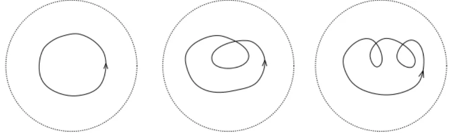
History of the problem. Consider the setWof allCrregular closed curves in the planeR2(i.e., CrimmersionsS1→R2), furnished with theCrtopology (r≥1). The Whitney-Graustein theorem ([24], thm. 1) states that two such curves are homotopic through regular closed curves if and only if they have the same rotation number (where the latter is the number of full turns of the tangent vector to the curve). Thus, the spaceWhas an infinite number of connected componentsWn, one for each rotation number n∈ Z. A typical element of Wn (n6= 0) is a circle traversed |n| times, with the direction depending on the sign ofn;W0 contains a figure eight curve.
For curves on the unit sphere S2 ⊂R3, there is no natural notion of rotation number. Indeed, the corresponding space I of Cr immersions S1 → S2 (i.e., regular closed curves on S2) has only two connected components, I+ and I−; this is an immediate consequence of a much more general result of S. Smale ([23], thm. A). The component I− contains all circles traversed an odd number of times, and the component I+ contains all circles traversed an even number of times. Actually, Smale’s theorem implies thatI± 'SO3×ΩS3, where ΩS3 denotes the set of all continuous closed
2010Mathematics Subject Classification. Primary: 53C42. Secondary: 57N20.
Key words and phrases. Curve; Geodesic curvature; Homotopy; Topology of infinite-dimensional manifolds.
1
arXiv:1304.2629v2 [math.GT] 4 Nov 2013
2 NICOLAU C. SALDANHA AND PEDRO Z ¨UHLKE
curves onS3, with the compact-open topology; the properties of the latter space are well understood (see [2],§16).†
In 1970, J. A. Little formulated and solved the following problem: Let C denote the set of all Cr closed curves onS2 which have nonvanishing geodesic curvature, with theCr topology (r≥2);
what are the connected components ofC? Although his motivation to investigateCappears to have been purely geometric, this space arises naturally in the study of a certain class of linear ordinary differential equations (see [20] for a discussion of this class and further references). In another notation, C is the space Free(S1,S2) of free closed spherical curves. A map f : M →N is called (second-order) free if the osculating space of order 2 is nondegenerate; forM =S1andN=S2, this is equivalent to saying that the curvef has nonvanishing geodesic curvature (cf. [6], [8]).
Little was able to show (see [13], thm. 1) that C has six connected components, C±1, C±2 and C±3, where the sign indicates the sign of the geodesic curvature of a curve in the corresponding component. A homeomorphism between Ci andC−i is obtained by reversing the orientation of the curves inCi.
Figure 1. The curves depicted above provide representatives of the components C1,C2andC3, respectively. All three are contained in the upper hemisphere ofS2; the dashed line represents the equator seen from above.
The topology of the spaceC has been investigated by quite a few other people since Little. We mention here only B. Khesin, B. Shapiro and M. Shapiro, who studiedC and similar spaces in the 1990’s (cf. [10], [11], [21] and [22]). They showed that C±1 are homotopy equivalent to SO3, and also determined the number of connected components of the spaces analogous to C inRn, Sn and RPn, for arbitraryn.
The first pieces of information about the homotopy and cohomology groups πk(C) and Hk(C) for k ≥1 were obtained a decade later by the first author in [16] and [17]. Finally, in the recent work [18], a description of the homotopy type of spaces of locally convex (but not necessarily closed) curves onS2 is presented. It is proved in particular that
C±2'SO3× ΩS3∨S2∨S6∨S10∨. . . and C±3'SO3× ΩS3∨S4∨S8∨S12∨. . .
.
The reason for the appearance of anSO3 factor in all of these results is that (unlike in [18]) we have not chosen a basepoint for the unit tangent bundle U TS2≈SO3; a careful discussion of this is given in §1.
Brief overview of this work. The main purpose of this work is to generalize Little’s theorem to other spaces of closed curves on S2. Let−∞ ≤ κ1 < κ2 ≤+∞be given and let Cκκ21 be the set of allCr closed curves onS2 whose geodesic curvatures are constrained to lie in the interval (κ1, κ2), furnished with theCrtopology (for somer≥2). In this notation, the spacesCandIdiscussed above becomeC0−∞tC+∞0 andC+∞−∞, respectively. Naturally, a space of curves onS2whose curvatures are constrained to lie in an open subset ofRis the disjoint union of spaces of this type.
We present a direct characterization of the connected components of Cκκ21 in terms of the pair κ1 < κ2 and of the properties of curves in Cκκ21. This yields a simple procedure to decide whether two given curves in Cκκ21 lie in the same component (that is, whether they are homotopic through
†The notationX'Y (resp.X≈Y) means thatX is homotopy equivalent (resp. homeomorphic) toY.
closed curves whose geodesic curvatures are constrained to (κ1, κ2)). Another consequence is that the number of components of Cκκ21 is always finite, and given by a simple formula involvingκ1,κ2.
More precisely, let ρi = arccot(κi), i = 1,2, where we adopt the convention that arccot takes values in [0, π], with arccot(+∞) = 0 and arccot(−∞) =π. Also, letbxcdenote the greatest integer smaller than or equal to x. ThenCκκ21 hasnconnected componentsC1, . . . ,Cn, where
(1) n=
π ρ1−ρ2
+ 1
and Cj contains circles traversed j times (1 ≤j ≤n). The component Cn−1 also contains circles traversed (n−1) + 2ktimes, andCncontains circles traversedn+ 2ktimes, fork∈N. Moreover, for n≥3, each ofC1, . . . ,Cn−2 is homeomorphic toSO3×E, whereE is the separable Hilbert space.
This result could be considered a first step towards the determination of the homotopy type of Cκκ21 in terms ofκ1andκ2. In this context, it is natural to ask whether the inclusionCκκ21 ,→C+∞−∞=I is a homotopy equivalence; as we have already mentioned, the topology of the latter space is well understood. It is shown in §10 of [25] that the answer is negative whenρ1−ρ2 ≤ 2π3 (note that ρ1−ρ2∈(0, π]), and we expect it to be negative except whenCκκ21 =C+∞−∞ (i.e., whenρ1−ρ2=π).
Actually, we conjecture thatCκκ21 andC¯κ¯κ21 have different homotopy types if and only ifρ1−ρ26=
¯
ρ1−ρ¯2, but here it will only be proved thatCκκ21 is homeomorphic toCκκ¯¯21 ifρ1−ρ2= ¯ρ1−ρ¯2(where ρi = arccotκi and ¯ρi = arccot ¯κi). Our guess is that the homotopy type of the “large” components Cn−1 andCn ofCκκ21 (withnas in (1)) is that of a space of the form
SO3× ΩS3∨S2n1∨S2n2∨S2n3∨. . . ,
n1≤n2≤n3≤ · · · being positive integers which can be obtained in terms ofκ1andκ2by formulas similar to (1).
Outline of the sections. It turns out that it is more convenient, but not essential, to work with curves which need not beC2. The curves that we consider possess continuously varying unit tangent vectors at all points, but their geodesic curvatures are defined only almost everywhere. This class of curves is described in§1, where we also relate the resulting spacesLκκ21 to the more familiar spaces Cκκ21 ofCrcurves: The inclusionCκκ21,→Lκκ21 is a homotopy equivalence and has dense image. In this section we take the first steps toward the main theorem by proving that the topology ofLκκ21depends only onρ1−ρ2. A corollary of this result is that any spaceLκκ21 is homeomorphic to a space of type L+∞κ0 ; the latter class is usually more convenient to work with. Some variations of our definition are also investigated. In particular, in this section we consider spaces of non-closed curves.
The main tools in the paper are introduced in§2. Given a curveγ∈L+∞κ0 , we assign toγcertain maps Bγ and Cγ, called the regular and caustic bands spanned by γ, respectively. These are “fat”
versions of the curve, which carry in geometric form important information on the curve. They are obtained by considering translations ofγ in the direction determined by its normal vector. We separate our curves into two main classes: If the image of the caustic band of a curve is contained in a hemisphere, the curve is called condensed; if this image contains two antipodal points, the curve is diffuse. Vaguely speaking, a condensed curve is one which does not wander too much aboutS2.
In §3, the grafting construction is introduced. Grafting a curve consists in cutting it at well chosen points, moving the resulting arcs and inserting new arcs in the gaps that arise (see fig. 7).
If the curve is diffuse, then we can graft arbitrarily long arcs of circles onto it. These are converted to loops, which are then spread along the curve (see fig. 6), so that it becomes loose in the sense that the constraints on the curvature become irrelevant. As a result, it is possible to deform it into a circle traversed a certain number of times, which is the canonical curve in our spaces.
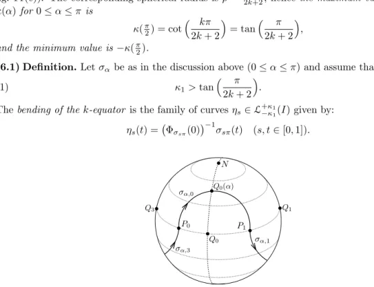
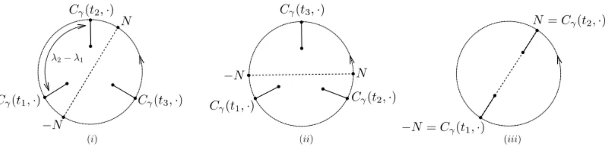
We reach the same conclusion for condensed curves in§4, where a notion of rotation number for curves of this type is also introduced: Ifγ is condensed, then we consider the set of all hemispheres which contain the image of its caustic band. Any such hemisphere is uniquely determined by a unit vector. Taking the average, we obtain a distinguished hemisphere, corresponding to some hγ ∈S2, containing Im(Cγ). Thishγ depends continuously onγ. The rotation numberν(γ) ofγis defined as the opposite of the usual rotation number of the image ofγ under stereographic projection through
−hγ. Forκ0<0, the proof thatγ∈L∞κ0 may be deformed into a circle involves a generalization of
4 NICOLAU C. SALDANHA AND PEDRO Z ¨UHLKE
the regular band of a curve, and forκ0≥0 the tools are M¨obius transformations and a version of the Whitney-Graustein theorem. Actually, it will be seen that the set of condensed curves in L+∞κ0
having a fixed rotation number is weakly homotopy equivalent to SO3, for anyκ0 (but it may not be a connected component).
Even though there exist curves which are neither condensed nor diffuse, any such curve is ho- motopic within L+∞κ0 to a curve of one of these two types. The results used to establish this are contained in §5. There, a more abstract version of rotation number for non-diffuse curves is intro- duced, and a bound on the total curvature of a non-diffuse curve inL+∞κ0 which depends only onκ0 and its rotation number is obtained. This is used to deduce that, by grafting the curve indefinitely, we must obtain either a condensed or a diffuse curve.
In§6 we decide when it is possible to deform a circle traversedktimes into a circle traversedk+ 2 times inL+∞κ0 . It is seen that this is possible if and only ifk≥n−1 =j
π ρ0
k(whereρ0= arccotκ0), and an explicit homotopy when this is the case is presented. It is also shown that the set of condensed curves inL+∞κ0 with fixed rotation numberk < n−1 is a connected component of this space (n≥3).
The proofs of the main theorems are given in§7, after most of the work has been done. We also obtain the following direct characterization of the components. Let ρ0 = arccotκ0, n =j
π ρ0
k + 1 andσbe the sign of (−1)n. Thenγ∈L+∞κ0 lies in:
(i) Lj if and only if it is condensed and has rotation numberj (1≤j≤n−2).
(ii) Ln−1if and only ifγ∈I−σand either it is non-condensed or condensed with rotation number ν(γ)≥n−1.
(iii) Ln if and only if γ∈Iσ and either it is non-condensed or condensed with rotation number ν(γ)≥n−1.
Here I± are the two components ofI =C+∞−∞, and Lj is the connected component of L+∞κ0 which contains circles traversedj times,j= 1, . . . , n. In particular, this yields a simple criterion to decide whether two curves γ1, γ2 ∈ Lκκ21 are homotopic within this space, provided only that we have parametrizations ofγ1andγ2.
Finally, some basic results on convexity in Sn (none of which is new) that are used throughout the work are collected in an appendix.
Acknowledgements. The content of this paper is essentially contained in the Ph.D. thesis [25] of the second author, who was advised by the first. Both authors gratefully acknowledge the financial support of cnpq,capesandfaperj, particularly during the second author’s graduate studies. We thank the members of the Ph.D. committee for several interesting suggestions. Very special thanks go to Boris Shapiro for helpful conversations with the first author during his visit to Stockholm Uni- versity, which inspired the main problem considered in this work. Finally, we thank the anonymous referee and Y. Eliashberg for their useful suggestions and comments.
1. Spaces of Curves on the Sphere with Constrained Geodesic Curvature Basic definitions and notation. LetM denote either the euclidean spaceRn+1or the unit sphere Sn ⊂ Rn+1, for some n ≥ 1. By a curve γ in M we mean a continuous map γ: [a, b] → M. A curve will be calledregular when it has a continuous and nonvanishing derivative; in other words, a regular curve is a C1 immersion of [a, b] intoM. For simplicity, the interval where γis defined will usually be [0,1].
Letγ: [0,1]→S2be a regular curve and let| |denote the usual Euclidean norm. Thearc-length parameter sofγis defined by
s(t) = Z t
0
|γ(t)|˙ dt, andL=R1
0 |γ(t)|˙ dtis called thelengthofγ. Derivatives with respect totandswill be systematically denoted by a ˙ and a0, respectively; this convention extends to higher-order derivatives as well.
Up to homotopy, we can always assume that a family of curves is parametrized proportionally to arc-length.
(1.1) Lemma. Let Abe a topological space and let a7→γa be a continuous map from A to the set of all Cr regular curvesγ: [0,1]→M (r≥1)with the Cr topology. Then there exists a homotopy γau: [0,1]→M,u∈[0,1], such that for any a∈A:
(i) γa0=γa andγa1 is parametrized so that|γ˙a1(t)|is independent oft.
(ii) γau is an orientation-preserving reparametrization ofγa, for allu∈[0,1].
Proof. Letsa(t) =Rt
0|γ˙a(τ)|dτ be the arc-length parameter ofγa, La its length andτa: [0, La]→ [0,1] the inverse function of sa. Defineγau: [0,1]→M by:
γau(t) =γa (1−u)t+uτa(Lat)
(u, t∈[0,1], a∈A).
Thenγau is the desired homotopy.
The unit tangent vector toγ at γ(t) will always be denoted by t(t). Set M =S2 for the rest of this section, and define theunit normal vector ntoγby
n(t) =γ(t)×t(t), where×denotes the vector product inR3.
Assume now that γ has a second derivative. By definition, thegeodesic curvature κ(s) ofγ at γ(s) is given by
(1) κ(s) =ht0(s),n(s)i.
Note that the geodesic curvature is not altered by an orientation-preserving reparametrization of the curve, but its sign is changed if we use an orientation-reversing reparametrization. Since the principal curvatures at any point of the sphere equal 1, the normal curvature ofγ is also identically equal to 1. In particular, its Euclidean curvatureK,
K(s) =p
1 +κ(s)2, never vanishes.
Closely related to the geodesic curvature of a curve γ: [0,1]→S2is theradius of curvature ofγ atγ(t), which we define as the unique numberρ(t)∈(0, π) satisfying
cotρ(t) =κ(t).
Note that the sign ofκ(t) is equal to the sign of π2 −ρ(t).
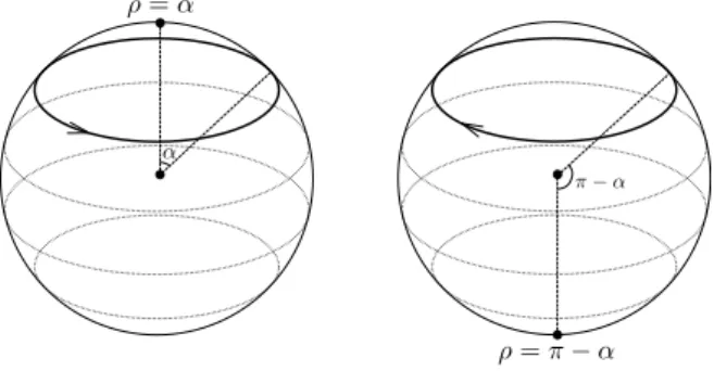
Example. A parallel circle of colatitude α, for 0< α < π, has geodesic curvature ±cotα(the sign depends on the orientation), and radius of curvature αor π−α at each point. (Recall that the colatitude of a point measures its distance from the north pole along S2.) The radius of curvature ρ(t) of an arbitrary curveγgives the size of the radius of the osculating circle toγatγ(t), measured alongS2and taking the orientation ofγinto account.
Figure 2. A parallel circle of colatitude α has radius of curvature α or π−α, depending on its orientation. We adopt the convention that the center (on S2) of a circle lies to its left, hence in the first figure the center is taken to be the north pole, and in the second, the south pole.
6 NICOLAU C. SALDANHA AND PEDRO Z ¨UHLKE
If we consider γ as a curve in R3, then its “usual” radius of curvature R is defined by R(t) =
1
K(t) = sinρ(t). We will rarely mention R or K again, preferring instead to work with ρ and κ, which are their natural intrinsic analogues in the sphere.
Spaces of curves. Given p∈S2 and v ∈TpS2 of norm 1, there exists a uniqueQ∈SO3 having p∈R3 as first column andv ∈ R3 as second column. We obtain thus a diffeomorphism between SO3and the unit tangent bundleU TS2 ofS2.
(1.2) Definition.For a regular curve γ: [0,1]→S2, itsframe Φγ: [0,1]→SO3 is the map given by
Φγ(t) =
| | |
γ(t) t(t) n(t)
| | |
.†
In other words, Φγ is the curve in U TS2 associated withγ, under the identification ofU TS2 with SO3. We emphasize that it is not necessary that γhave a second derivative for Φγ to be defined.
Now let −∞ ≤ κ1 < κ2 ≤+∞ and Q∈SO3. We would like to study the space Lκκ21(Q) of all regular curves γ: [0,1]→S2satisfying:
(i) Φγ(0) =I and Φγ(1) =Q;
(ii) κ1< κ(t)< κ2 for eacht∈[0,1].
Here I is the 3×3 identity matrix and κis the geodesic curvature ofγ. Condition (i) says that γ starts ate1 in the directione2 and ends atQe1 in the directionQe2.
This definition is incomplete because we have not described the topology of Lκκ21(Q). The most natural choice would be to require that the curves in this space be of classC2, and to give it theC2 topology. The foremost reason why we will not follow this course is that we would like to be able to perform some constructions which yield curves that are notC2. We shall adopt a more complicated definition in order to avoid using convolutions or other tools all the time to smoothen a curve.
(1.3) Definition.A functionf: [a, b]→Ris said to be of classH1if it is an indefinite integral of someg∈L2[a, b]. We extend this definition to mapsF: [a, b]→Rn by saying thatF is of classH1 if and only if each of its component functions is of classH1.
Since L2[a, b] ⊂L1[a, b], an H1 function is absolutely continuous (and differentiable almost ev- erywhere).
We shall now present an explicit description of a topology onLκκ21(Q) which turns it into a Hilbert manifold. The definition is unfortunately not very natural. However, we shall prove the following two results relating this space to more familiar concepts: First, for any r ∈N, r ≥2, the subset of Lκκ21(Q) consisting ofCr curves will be shown to be dense in Lκκ21(Q). Second, we will see that the space of Cr regular curves satisfying conditions (i) and (ii) above, with the Cr topology, is homeomorphic toLκκ21(Q).‡
Consider first a smooth regular curveγ: [0,1]→S2. From the definition of Φγ we deduce that (2) Φ˙γ(t) = Φγ(t)Λ(t), where Λ(t) =
0 − |γ(t)|˙ 0
|γ(t)|˙ 0 − |γ(t)|˙ κ(t) 0 |γ(t)|˙ κ(t) 0
∈so3
is called thelogarithmic derivative of Φγ andκis the geodesic curvature ofγ.
Conversely, givenQ0∈SO3 and a smooth map Λ : [0,1]→so3 of the form
(3) Λ(t) =
0 −v(t) 0 v(t) 0 −w(t)
0 w(t) 0
,
†In previous works of the first author, this is denoted byFγ and called theFrenet frame ofγ. We will not use this terminology to avoid any confusion with the usual Frenet frame ofγwhen it is considered as a curve inR3.
‡The definitions given here are straightforward adaptations of the ones in [19], where they are used to study spaces of locally convex curves inSn(which correspond to the spacesL+∞0 (Q) whenn= 2).
let Φ : [0,1]→SO3 be the unique solution to the initial value problem
(4) Φ(t) = Φ(t)Λ(t),˙ Φ(0) =Q0.
Define γ: [0,1]→S2 to be the smooth curve given byγ(t) = Φ(t)e1. Thenγ is regular if and only ifv(t)6= 0 for allt∈[0,1], and it satisfies Φγ = Φ if and only ifv(t)>0 for allt. (Ifv(t)<0 for all tthenγ is regular, but Φγ is obtained from Φ by changing the sign of the entries in the second and third columns.)
Equation (4) still has a unique solution if we only require thatv, w∈L2[0,1] (cf. [4], p. 67). With this in mind, let E=L2[0,1]×L2[0,1] and leth: (0,+∞)→Rbe the smooth diffeomorphism
(5) h(t) =t−t−1.
For each pairκ1< κ2∈R, lethκ1, κ2: (κ1, κ2)→Rbe the smooth diffeomorphism hκ1, κ2(t) = (κ1−t)−1+ (κ2−t)−1
and, similarly, set
h−∞,+∞:R→R h−∞,+∞(t) =t
h−∞,κ2: (−∞, κ2)→R h−∞,κ2(t) =t+ (κ2−t)−1 hκ1,+∞: (κ1,+∞)→R hκ1,+∞(t) =t+ (κ1−t)−1.
(1.4) Definition.Let κ1, κ2 satisfy−∞ ≤ κ1 < κ2 ≤+∞. A curveγ: [0,1]→ S2 will be called (κ1, κ2)-admissible if there exist Q0 ∈ SO3 and a pair (ˆv,w)ˆ ∈ E such that γ(t) = Φ(t)e1 for all t∈[0,1], where Φ is the unique solution to equation (4), withv, wgiven by
(6) v(t) =h−1(ˆv(t)), w(t) =v(t)h−1κ1, κ2( ˆw(t)).
When it is not important to keep track of the bounds κ1, κ2, we shall say more simply thatγ is admissible.
In vague but more suggestive language, an admissible curveγis essentially anH1frame Φ : [0,1]→ SO3such thatγ= Φe1: [0,1]→S2has geodesic curvature in the interval (κ1, κ2). The unit tangent (resp. normal) vector t(t) = Φ(t)e2 (resp.n(t) = Φ(t)e3) of γ is thus defined everywhere on [0,1], and it is absolutely continuous as a function oft. The curveγitself is, like Φ, of classH1. However, the coordinates of its velocity vector ˙γ(t) =v(t) Φ(t)e2 lie inL2[0,1], so the latter is only defined almost everywhere. The geodesic curvature ofγ, which is also defined a.e., is given by
κ(t) = 1 v(t)
t(t),˙ n(t)
=w(t) v(t) =h−1κ
1, κ2( ˆw(t))∈(κ1, κ2)
(cf. (2), (3) and (6)). Note also that if we parametrizeγby (a multiple of) its arc-length parameter instead, then it becomes a C1 curve, for thenγ0 =tis absolutely continuous.
Remark. The reason for the choice of the specific diffeomorphism h: (0,+∞) →R in (5) (instead of, say, h(t) = logt) is that we needh−1(t) to diverge linearly to ±∞ as t → 0,+∞ in order to guarantee that v=h−1◦vˆ∈L2[0,1] whenever ˆv∈L2[0,1]. The reason for the choice of the other diffeomorphisms is analogous.
(1.5) Definition.Let −∞ ≤ κ1 < κ2 ≤ +∞, Q0 ∈ SO3. Define Lκκ21(Q0,·) to be the set of all (κ1, κ2)-admissible curvesγ such that
Φγ(0) =Q0,
where Φγ is the frame of γ. This set is identified withE via the correspondenceγ ↔ (ˆv,w), andˆ this defines a (trivial) Hilbert manifold structure onLκκ21(Q0,·).
In particular, this space is contractible by definition. We are now ready to define the spaces Lκκ21(Q), which constitute the main object of study of this work.
8 NICOLAU C. SALDANHA AND PEDRO Z ¨UHLKE
(1.6) Definition.Let −∞ ≤κ1 < κ2 ≤+∞, Q∈SO3. We define Lκκ21(Q) to be the subspace of Lκκ21(I,·) consisting of all curvesγ in the latter space satisfying
(i) Φγ(0) =I and Φγ(1) =Q.
Here Φγ is the frame ofγandI is the 3×3 identity matrix.†
BecauseSO3 has dimension 3, the condition Φγ(1) =Qimplies thatLκκ21(Q) is a closed subman- ifold of codimension 3 in E≡Lκκ21(I,·). (Here we are using the fact that the map which sends the pair (ˆv,w)ˆ ∈E to Φ(1) is a submersion; a proof of this whenκ1= 0 andκ2= +∞can be found in
§3 of [18], and the proof of the general case is analogous.) The spaceLκκ21(Q) consists of closed curves only whenQ =I. Also, when κ1 =−∞ andκ2 = +∞simultaneously, no restrictions are placed on the geodesic curvature. The resulting space (for arbitrary Q∈SO3) is known to be homotopy equivalent to ΩS3tΩS3; see the discussion after (1.14).
Note that we have natural inclusions Lκκ21(Q) ,→ L¯κ¯κ21(Q) whenever ¯κ1 ≤ κ1 < κ2 ≤ κ¯2. More explicitly, this map is given by:
γ≡(ˆv,w)ˆ 7→ v, hˆ κ¯1,¯κ2◦h−1κ1,κ2( ˆw)
;
it is easy to check that the actual curve associated with the pair of functions in Lκκ¯¯21(Q) on the right side (via (3), (4) and (6)) is the original curve γ, so that the use of the term “inclusion” is justified. We remark that although it is a continuous injection, it is not a topological embedding unless ¯κ1=κ1 and ¯κ2=κ2.
(1.7) Lemma. LetM,Nbe Banach manifolds. Then:
(a) M is locally path-connected. In particular, its connected components and path components coincide.
(b) IfM,Nare weakly homotopy equivalent, then they are in fact homeomorphic (diffeomorphic if M,Nare Hilbert manifolds). In particular, ifMis weakly contractible, then it is contractible.
(c) LetEandFbe separable Banach spaces. Supposei:F→Eis a bounded, injective linear map with dense image and M⊂E is a smooth closed submanifold of finite codimension. Then N =i−1(M) is a smooth closed submanifold of F and i: (F,N) → (E,M) is a homotopy equivalence of pairs.
Proof. Part (a) is obvious. Part (b) follows from thm. 15 in [15] and cor. 3 in [9]. Part (c) is thm. 2
in [3].
(1.8) Lemma. LetEbe a separable Hilbert space,D⊂Ea dense vector subspace,L⊂Ea subman- ifold of finite codimension and U an open subset ofL. Then the set inclusion D∩U →U induces surjections on homotopy groups.
Proof. We shall prove the lemma whenL=h−1(0) for some submersionh:V →Rn, whereV is an open subset ofE. This is sufficient for our purposes and the general assertion can be deduced from this by using a partition of unity subordinate to a suitable cover of Lby convex open sets.
LetT be a tubular neighborhood ofUinV. LetKbe a compact simplicial complex andf:K→U a continuous map. We shall obtain a continuous H: [0,2]×K →U such thatH(0, a) =f(a) for everya∈KandH({2} ×K)⊂D∩U. Letej denote thej-th vector in the canonical basis forRn, e0 =−Pn
j=1ej and let ∆ ⊂Rn denote the n-simplex [e0, . . . , en]. Let [x0, x1, . . . , xn] ⊂T be an n-simplex and ϕ: ∆→[x0, x1, . . . , xn] be given by
ϕ n
X
j=0
sjej
=
n
X
j=0
sjxj, where
n
X
j=0
sj= 1 and sj ≥0 for all j= 0, . . . , n.
We shall say that [x0, x1, . . . , xn] isgood ifh◦ϕ: ∆→T is a diffeomorphism and 0∈(h◦ϕ)(Int ∆).
Givenp∈T, letdhp denote the derivative ofhatpand Np= ker(dhp). Definewj:T →Eby:
(7) wj(p) = dhp|N⊥
p
−1
(ej) (p∈T, j= 0, . . . , n).
†The letter ‘L’ inLκκ21(Q) is a reference to John A. Little, who determined the connected components ofL+∞0 (I) in [13].
Notice that when|λj|is small for eachj, we haveh(p+P
jλjwj(p))≈P
jλjej. Using compactness ofK, we can findr, ε >0 such that:
(i) For any p∈f(K), [p+rw0(p), . . . , p+rwn(p)]⊂T and it is good;
(ii) If p∈f(K) and|qj−(p+rwj(p))|< εfor eachj, then [q0, . . . , qn]⊂T and it is good.
Letai (i= 1, . . . , m) be the vertices of the triangulation of K. Setvi=f(ai) and vij =vi+rwj(vi) (i= 1, . . . , m, j= 0, . . . , n).
For each suchi, j, choose ˜vij∈D∩T with|˜vij−vij|< ε2. Let vij(s) = (2−s)vij+ (s−1)˜vij, so that
|vij(s)−vij|<ε
2 (s∈[1,2], i= 1, . . . , m, j= 0, . . . , n).
(8)
For anyi, i0∈ {1, . . . , m}andj = 0, . . . , n, we have
|vij−vi0j| ≤ |f(ai)−f(ai0)|+r|wj◦f(ai)−wj◦f(ai0)|.
Sincef and thewj are continuous functions, we can suppose that the triangulation ofK is so fine that |vij−vi0j| < ε2 for eachj = 0, . . . , n whenever there exists a simplex having ai, ai0 as two of its vertices. Let a∈K lie in somed-simplex of this triangulation, say, a=Pd+1
i=1tiai (where each ti>0 andP
iti= 1). Set
zj(s) =
d+1
X
i=1
tivij(s) (s∈[1,2], j= 0, . . . , n).
Then [z0(s), . . . , zn(s)] is a good simplex because condition (ii) is satisfied (withp=v1):
d+1
X
i=1
tivij(s)−v1j
≤
d+1
X
i=1
ti |vij(s)−vij|+|vij−v1j|
< ε,
where the strict inequality comes from (8) and our hypothesis on the triangulation. DefineH(s, a) as the unique element of h−1(0)∩[z0(s), . . . , zn(s)] (s∈ [1,2]). Note that H(2, a) is some convex combination of the ˜vij ∈D, henceH(2, a)∈D∩U for alla∈K.
By reducingr, ε >0 (and refining the triangulation ofK) if necessary, we can ensure that (1−s)f(a) +sH(1, a)∈T for alls∈[0,1] anda∈K.
Let pr :T →U be the associated retraction. Complete the definition ofH by setting:
H(s, a) = pr (1−s)f(a) +sH(1, a)
∈T (s∈[0,1],a∈K).
The existence of H shows that f is homotopic within U to a map whose image is contained in D∩U. TakingK = Sk, we conclude that the set inclusion D∩U → U induces surjective maps
πk(D∩U)→πk(U) for allk∈N.
(1.9) Lemma. Let r∈ {2,3, . . . ,∞}. Then the subset of all γ: [0,1]→S2 of class Cr is dense in Lκκ21(Q).
Proof. This follows from the previous lemma by taking E = L2[0,1]×L2[0,1], D = C∞[0,1]×
C∞[0,1] andU any open subset ofL=Lκκ21(u, v).
(1.10) Definition.Let−∞ ≤ κ1< κ2 ≤+∞, Q∈SO3 and r∈N, r ≥2. Define Cκκ21(Q) to be the set, furnished with theCr topology, of allCr regular curvesγ: [0,1]→S2 such that:
(i) Φγ(0) =I and Φγ(1) =Q;
(ii) κ1< κ(t)< κ2 for eacht∈[0,1].
Notice that these spaces are Banach manifolds. The value ofris not important, in the sense that different values of r yield homeomorphic spaces. Because of this, after the next lemma, when we speak ofCκκ21(Q), we will implicitly assume thatr= 2.
(1.11) Lemma.Let r ∈N (r≥2),Q∈SO3 and−∞ ≤κ1 < κ2 ≤+∞. Then the set inclusion i:Cκκ21(Q),→Lκκ21(Q)is a homotopy equivalence. Therefore,Cκκ21(Q)andLκκ21(Q)are homeomorphic.
10 NICOLAU C. SALDANHA AND PEDRO Z ¨UHLKE
Proof. In this proof we will highlight the differentiability class by denotingCκκ21(Q) byCκκ21(Q)r. Let E = L2[0,1]×L2[0,1], let F = Cr−1[0,1]×Cr−2[0,1] (where Ck[0,1] denotes the set of all Ck functions [0,1]→R, with theCk norm) and leti:F→E be set inclusion. SettingM=Lκκ21(Q), we conclude from (1.7 (c)) thati:N=i−1(M),→Mis a homotopy equivalence. We claim thatNis homeomorphic toCκκ21(Q)r, where the homeomorphism is obtained by associating a pair (ˆv,w)ˆ ∈N to the curveγ obtained by solving (4) (with Λ defined by (3) and (6) andQ0=I), and vice-versa.
Suppose first that γ ∈ Cκκ21(Q)r. Then |γ|˙ (resp. κ) is a function [0,1] → R of class Cr−1 (resp.Cr−2). Hence, so are ˆv=h◦ |γ|˙ and ˆw=hκκ21◦κ, sincehandhκκ21 are smooth. Conversely, if (ˆv,w)ˆ ∈N, thenv =h−1◦vˆis of classCr−1 andw= (hκκ21)−1◦wˆ of class Cr−2, and the frame Φ of the curveγcorresponding to that pair satisfies
Φ = ΦΛ,˙ Λ =
0 − |γ|˙ 0
|γ|˙ 0 − |γ|˙ κ 0 |γ|˙ κ 0
=
0 −v 0
v 0 −w
0 w 0
.
Since the entries of Λ are of class (at least) Cr−2, the entries of Φ are functions of class Cr−1. Moreover,γ= Φe1, hence
˙
γ= ˙Φe1= ΦΛe1=vΦe2,
and the velocity vector of γ is seen to be of class Cr−1. It follows that γ is a curve of class Cr. Finally, it is easy to check that the correspondence (ˆv,w)ˆ ↔γis continuous in both directions.
The last assertion follows from (1.7 (b)).
Lifted frames. The (two-sheeted) universal covering space ofSO3 isS3. Let us briefly recall the definition of the covering map π: S3 → SO3.† We start by identifying R4 with the algebra H of quaternions, and S3 with the subgroup of unit quaternions. Given z ∈ S3, v ∈ R4, define a transformationTz: R4→R4byTz(v) =zvz−1=zvz. One checks easily thatTzpreserves the sum, multiplication and conjugation operations. It follows that, for anyv, w∈R4,
4hTz(v), Tz(w)i=|Tz(v) +Tz(w)|2− |Tz(v)−Tz(w)|2
=|v+w|2− |v−w|2= 4hv, wi,
whereh,idenotes the usual inner product inR4. ThusTzis an orthogonal linear transformation of R4. Moreover,Tz(1) =1(where 1is the unit ofH), hence the three-dimensional vector subspace {0} ×R3 ⊂R4 consisting of the purely imaginary quaternions is invariant underTz. The element π(z) ∈ SO3 is the restriction of Tz to this subspace, where (a, b, c) ∈ R3 is identified with the quaternionai+bj+ck.
In what follows we adopt the convention that S3 (resp.SO3) is furnished with the Riemannian metric inherited fromR4 (resp.R9).
(1.12) Lemma.Let h,idenote the metric in S3 andhhh,iii the metric in SO3. Thenπ∗hhh,iii= 8h,i, whereπ∗hhh,iii denotes the pull-back ofhhh,iiiby π.
Proof. The proof is a straightforward calculation. The details may be found in [25], (2.11).
(1.13) Definition.Let Φγ: [0,1] → SO3 be the frame of an admissible curve γ and let z ∈ S3 satisfyπ(z) = Φγ(0). We define the lifted frame Φ˜zγ: [0,1]→S3 to be the lift of Φγ toS3, starting at z. When Φγ(0) =I we adopt the convention that z=1, and we denote the lifted frame simply by ˜Φγ.
Here is a simple but important application of this concept.
(1.14) Lemma.Let γ0, γ1 ∈Lκκ21(Q), for some Q ∈SO3, and suppose that γ0, γ1 lie in the same connected component of this space. ThenΦ˜γ0(1) = ˜Φγ1(1).
†See [5] for more details and further information on quaternions and rotations.
Proof. SinceLκκ21(Q) is a Hilbert manifold, its path and connected components coincide. Therefore, to say that γ0, γ1 lie in the same connected component of Lκκ21(Q) is the same as to say that there exists a continuous family of curves γs ∈ Lκκ21(Q) joining γ0 and γ1, s ∈ [0,1]. The family Φγs yields a homotopy between the paths Φγ0 and Φγ1 in SO3. (Recall that each of the frames Φγs is (absolutely) continuous.) By the homotopy lifting property of covering spaces, the paths ˜Φγ0 and
Φ˜γ1 are also homotopic inS3(fixing the endpoints).
The role of the initial and final frames. We will now study how the topology ofLκκ21(Q) changes if we consider variations of condition (i) in (1.6); by the end of the section it should be clear that our original definition is sufficiently general. A summary of all the definitions considered here is given in table form on p. 14.
For fixedz∈S3, let ΩzS3denote the set of all continuous pathsω: [0,1]→S3such thatω(0) =1 and ω(1) = z, furnished with the compact-open topology. It can be shown (see [2], p. 198) that ΩzS3'ΩS3for anyz∈S3, where ΩS3 is the space of paths inS3 which start and end at1∈S3.† The topology of this space is well understood; we refer the reader to [2],§16, for more information.
Now letκ1< κ2,z∈S3be arbitrary andQ=π(z). Define
(9) F:Lκκ21(Q)→ΩzS3∪Ω−zS3'ΩS3tΩS3 by F(γ) = ˜Φγ.
In the special caseκ1=−∞,κ2= +∞, it follows from the Hirsch-Smale theorem (see [23], thm. C) that this map is a weak homotopy equivalence. In the general case this is false, however. For instance, ΩS3tΩS3 has two connected components, while Little has proved ([13], thm. 1) that L+∞0 (I) has three connected components. We take this opportunity to recall the precise statement of Little’s theorem and to introduce a new class of spaces.
(1.15) Definition.Let−∞ ≤κ1< κ2≤+∞. DefineLκκ21 to be the space of all (κ1, κ2)-admissible curvesγ: [0,1]→S2 such that
Φγ(0) = Φγ(1).
Note that the only difference betweenLκκ21(I) andLκκ21 is that curves in the latter space may have arbitrary initial and final frames, as long as they coincide. An argument analogous to the one given for the spaces Lκκ21(Q) shows that Lκκ21 is also a Hilbert manifold. In fact, we have the following relationship between the two classes.
(1.16) Proposition.The spaceLκκ21 is homeomorphic toSO3×Lκκ21(I).
Proof. ForQ∈ SO3 and γ ∈Lκκ21(I), let Qγ be the curve defined by (Qγ)(t) =Q(γ(t)). Because Q is an isometry, the geodesic curvatures of Qγ at (Qγ)(t) and of γ at γ(t) coincide. Define F:SO3×Lκκ21(I)→ Lκκ21 by F(Q, γ) = Qγ; clearly, F is continuous. Since it has the continuous
inverseη7→(Φη(0),Φη(0)−1η),F is a homeomorphism.
Let us temporarily denote byLthe spaceL0−∞tL+∞0 studied by Little. We haveL0−∞≈L+∞0 , since the map which takes a curve inLto the same curve with reversed orientation is a (self-inverse) homeomorphism mapping L0−∞ onto L+∞0 . What is proved in [13] is that L has six connected components.‡ Using prop. (1.16) and the fact thatSO3is connected, we see that Little’s theorem is equivalent to the assertion thatL+∞0 (I) has three connected components, as was claimed immediately above (1.15).
A natural generalization of the spaces Lκκ21(Q) is obtained by modifying condition (i) of (1.6) as follows.
(1.17) Definition.Let −∞ ≤κ1 < κ2 ≤+∞ andQ0, Q1 ∈SO3. Define Lκκ21(Q0, Q1) to be the space of all (κ1, κ2)-admissible curvesγ: [0,1]→S2such that
(i0) Φγ(0) =Q0 and Φγ(1) =Q1.
Thus, the only difference between condition (i) on p. 8 and condition (i0) is that the latter allows arbitrary initial frames.
†The notationX'Y (resp.X≈Y) means thatX is homotopy equivalent (resp. homeomorphic) toY.
‡Little works withC2curves, but, as we have seen, this is not important.
12 NICOLAU C. SALDANHA AND PEDRO Z ¨UHLKE
(1.18) Proposition.Let P, Q0, Q1 ∈SO3. Then Lκκ21(Q0, Q1)≈ Lκκ21(P Q0, P Q1). In particular, Lκκ21(Q0, Q1)≈Lκκ21(Q), whereQ=Q−10 Q1.
Proof. The proof is similar to that of (1.16). The mapγ7→P γtakesLκκ21(Q0, Q1) intoLκκ21(P Q0, P Q1) and is continuous. The map γ7→P−1γ, which is likewise continuous, is its inverse.
Of course, we could also consider the spacesLκκ21(·, Q), consisting of all (κ1, κ2)-admissible curves γ having final frame Φγ(1) =Q∈ SO3 (but arbitrary initial frame). LikeLκκ21(Q,·), this space is contractible. To see this, one can go through the definition to check that it is indeed homeomor- phic to E, or, alternatively, one can observe that the map γ 7→ ¯γ, ¯γ(t) = γ(1−t), establishes a homeomorphism
Lκκ21(·, Q)≈Lκκ21(QR,·), where
R=
1 0 0
0 −1 0
0 0 −1
.
Finally, we could study the spaceLκκ21(·,·) of all (κ1, κ2)-admissible curves, with no conditions placed on the frames. The argument given in the proof of (1.16) shows that
Lκκ21(·,·)≈SO3×Lκκ21(I,·).
Hence,Lκκ21(·,·) is homeomorphic toSO3×E, and has the homotopy type ofSO3.
Thus, the topology of the spaces Lκκ21(Q,·),Lκκ21(·, Q) andLκκ21(·,·) is uninteresting. We will have nothing else to say about these spaces.
The role of the bounds on the curvature. Having analyzed the significance of condition (i) on p. 6, let us examine next condition (ii). Notice that we have allowed the boundsκ1,κ2 on the curvature to be infinite. The definition of radius of curvature is extended accordingly by setting arccot(+∞) = 0 and arccot(−∞) =π. We can then rephrase (ii) as:
(ii) ρ(t)∈(ρ2, ρ1) for eacht∈[0,1].
Here ρis the radius of curvature of γ and ρi = arccotκi ∈[0, π], i = 1,2. The main result of this section relates the topology of Lκκ21(Q) to the sizeρ1−ρ2 of the interval (ρ2, ρ1). Its proof relies on the following construction.
Given −π < θ < π and an admissible curveγ: [0,1]→S2, define thetranslation γθ: [0,1]→S2 ofγ byθ to be the curve given by
(10) γθ(t) = cosθ γ(t) + sinθn(t) (t∈[0,1]).
Example. Let 0< α < π2 and letC be the circle of colatitudeα. Depending on the orientation, the translation of C byθ, 0≤θ ≤α, is either the circle of colatitude α+θ or the circle of colatitude α−θ. In particular, takingθ=αand a suitable orientation ofC, the translation degenerates to a single point (the north pole).
This example shows that some care must be taken in the choice ofθfor the resulting curve to be admissible.
(1.19) Lemma.Let γ: [0,1]→S2 be an admissible curve and ρits radius of curvature. Suppose (11) ρ2< ρ(t)< ρ1 for a.e. t∈[0,1] and ρ1−π≤θ≤ρ2.
Thenγθ is an admissible curve and its frame is given by:
(12) Φγθ = ΦγRθ, where Rθ=
cosθ 0 −sinθ
0 1 0
sinθ 0 cosθ
.
![Figure 3. The number of connected components of L κ κ 2 1 , as ρ 1 − ρ 2 varies in (0, π]](https://thumb-eu.123doks.com/thumbv2/123dok_br/17632383.4198166/15.892.310.589.389.524/figure-number-connected-components-l-κ-κ-varies.webp)
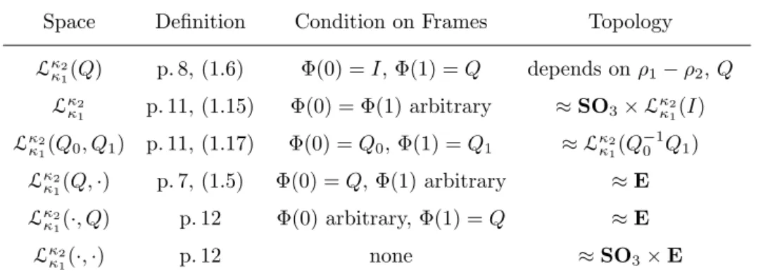
![Figure 5. A curve γ ∈ L +∞ κ 0 (Q) and the curve γ [t 0 #n] obtained from γ by adding loops at γ(t 0 ).](https://thumb-eu.123doks.com/thumbv2/123dok_br/17632383.4198166/22.892.263.642.478.697/figure-curve-γ-l-curve-obtained-adding-loops.webp)
![Figure 13. An illustration of the boundary of the rectangle R = B γ | [τ 0 ,τ 1 ]×[ρ 0 −π,0]](https://thumb-eu.123doks.com/thumbv2/123dok_br/17632383.4198166/43.892.365.521.216.407/figure-illustration-boundary-rectangle-r-b-γ-τ.webp)