Some of the best algorithms of the computer age are highlighted in the January/February 2000 issue of Computing in Science. amp; Engineering, a joint publication of the American Institute of Physics and the IEEE Computer Society. In terms of widespread use, Dantzig's algorithm is one of the most successful of all time: Linear programming dominates the world of industry, where economic survival depends on the ability to optimize within budget and other constraints. Iterative methods - such as solving equations of the form Kxi + 1 = Kxi + b - Axi with a simpler matrix K that is ideally "close" to A - lead to the study of Krylov subspaces.
It also facilitates the analysis of rounding errors, one of the great bugbears of numerical linear algebra. In 1961 James Wilkinson of the National Physical Laboratory in London published a seminal paper in the Journal of the ACM entitled "Error Analysis of Direct Methods of Matrix Inversion", based on the LU decomposition of a matrix as a product of under and top layers. triangular factors.). As Backus himself recalls in a recent history of Fortran I, II, and III published in 1998 in the IEEE Annals of the History of Computing, the compiler "produced code with such efficiency that its output would frighten the programmers who studied it ". .
If the Euclidean algorithm doesn't end - or if you just get tired of calculating it - then the unraveling procedure at least provides lower bounds on the size of the relation to the smallest integer. For example, their detection algorithm has been used to find the precise coefficients of the polynomials satisfied by the third and fourth bifurcation points, B and B, of the logistic map. This algorithm overcomes one of the major problems of N-body simulations: the fact that for accurate calculations of the motions of N particles interacting via gravitational or electrostatic forces (think stars in a galaxy or atoms in a protein) O(N2) calculations - one for each pair of particles.
One of the obvious advantages of the fast multipole algorithm is that it is equipped with rigorous error estimates, a feature that many methods lack.
An intuitive algebraic approach for solving Linear Programming problems”
Fundamentals and scope
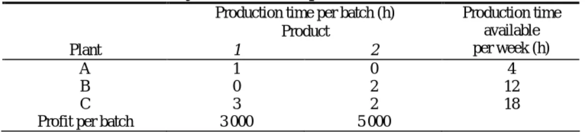
Based on a prototype example, linear programming and the simplex solution method are presented. The text is based on the book by Hillier and Lieberman [2005] and begins with segments of the third chapter of the book.
Explanation of the simplex method 3 Introduction to Linear Programming
- Prototype example
4 Solving Linear Programming problems
- Setting up the Simplex Method
- The algebra of the Simplex Method
- The Simplex Method in tabular form
- for the Example
- Tie breaking in the Simplex Method
- Adapting to other model forms
- Epilogue
- Acknowledgements
- References
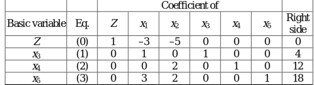
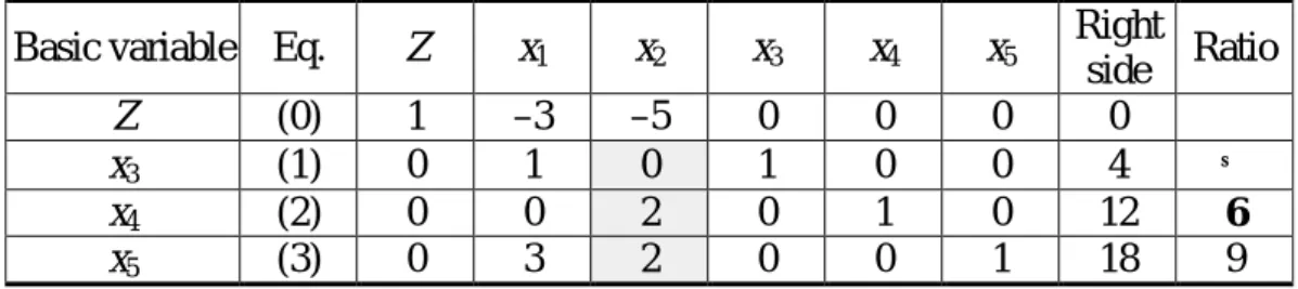
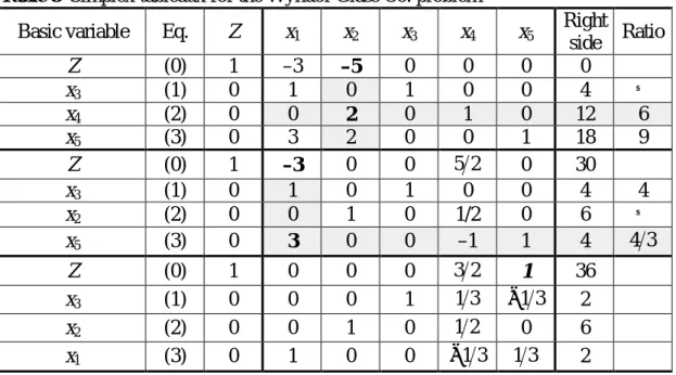
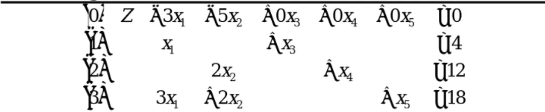
The non-basis variables (including the input variable) are non-negative, but we need to check how far x2 can be increased without violating the non-negativity constraints on the basic variables. In any iteration of the simplex method, Step 2 uses the minimum test ratio to determine which base variable falls to zero first as the input variable increases. Decreasing this base variable to zero will convert it to a non-base variable for the next BF solution.
That's why this variable is called the leaving variable for the current iteration (because it leaves the base). In addition, this form also identifies the values of x3 and x5 for the new solution. The tabular form of the simplex method records only the essential information, namely (1) the coefficients of the variables, (2) the constants on the right side of the equations, and (3) the base variable that appears in each equation.
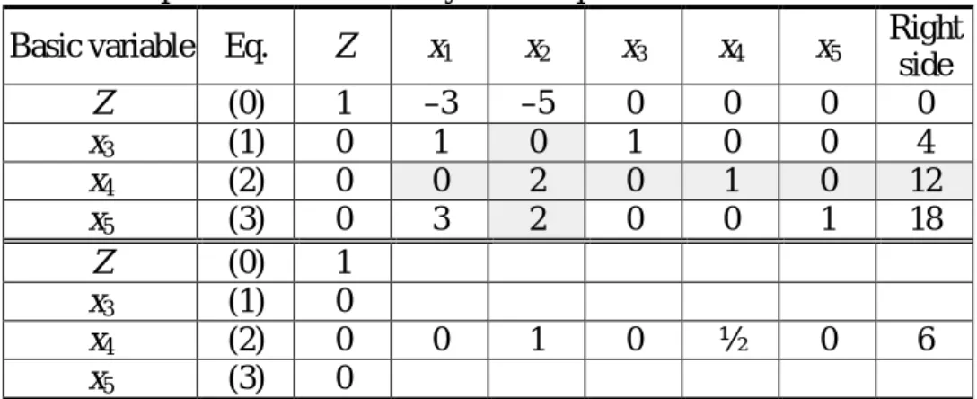
For the example, the calculations for the minimum ratio test are shown to the right of Table 4. Thus row 2 is the pivot row (shown in the first half of Table 5) and x4 is the outgoing base variable. Solve the new BF solution by using elementary row operations to construct a new simplex tableau in proper form from Gaussian elimination under the current one, then return to the optimality test.
For the Example: since x2 replaces x4 as a basic variable, we must reproduce the first tableau's pattern of coefficients in the column of x in the second tableau's column of x2. If two or more basic variables in an iteration are the remaining variable, it matters which one is chosen. First, all the linked variables reach zero simultaneously if the incoming basic variable is incremented.
Therefore, the one or those not chosen to be the left basic variable will also have a value of zero in the new solution. If a loop should occur, one can always get out by changing the choice of the departure basic variable. If the smallest nonnegative ratio does not exist, the solution to the objective function is unbounded (infinity).
Artificial variables in Linear Programming
Since the coefficient of x1 is the best (largest), this variable is chosen as the input variable.
Redundant ?
Impossible ?
A study was undertaken to determine the percentage of waste solids removed in a filtration system as a function of the flow rate, x, of the wastewater introduced into the system. It was decided to use a flow rate of 2(2)14 gal/min and to observe (“experimental”) the percentage of waste material removed when each of these flow rates was used.
Resolution
Uma solução inadmissível — matriz do transporte, X
Uma solução admissível («não-básica»)
Solução pelo «método de Vogel» ou «das diferenças» (— modificado)
Outra heurística: método de Vogel
Calcule, na matriz C restante, a diferença entre os dois valores menores em cada fila (linha ou coluna) e seleccione a fila que tiver a diferença máxima
Atribua, na matriz X, a quantidade maior possível ao elemento mais barato da fila seleccionada
- Verificar se há entrepostos
Na «reação em cadeia», apenas um dos quadrados decrescentes é cancelado (qualquer . — por exemplo, o mais barato); o restante fica com uma quantidade arbitrariamente pequena, ε. O critério de otimalidade "passo" (como é típico da programação linear, da qual é um caso específico) é uma condição suficiente, mas não necessária. Na matriz de custos assim aumentada foram adicionados: colunas de custos das viagens entre as origens e os armazéns adicionais; e linhas de custo para viagens entre armazéns e destinos adicionais.
O problema de «planeamento de produção»
Fazendo xij o número de motores produzidos no mês i para montagem no mês j e cij o custo correspondente, podemos criar o problema de transporte do Quadro 6A, ainda incompleto.
O problema da Afectação
Insert junctions — Transshipment points or depots or junctions (remaining)
Balance — If the transportation problem is not balanced, insert one fictitious source or destination with the capacity difference (and 0 transportation costs)