We conclude by assessing the current state of the art and trends for the future. With specific implementations of these elements, many different versions of the basic algorithm can be achieved. In the following sections, we discuss a number of the most common enhancements to these basic techniques.
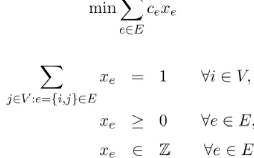
The performance of the branch-and-bound algorithm depends critically on the ability to compute bounds that are close to the value of the optimal solution. Considering only (4), we have a MILP relaxation, called the 0−1 knapsack problem, with a feasible region.
ABACUS .1 Overview
Compared to the similar MILP framework BCP, ABACUS has a slightly cleaner interface, with fewer classes and a more straightforward object-oriented structure. The target audience for ABACUS is advanced users who need a powerful framework for implementing advanced versions of branch and bound, but don't need a callable library interface. There are four major C++ base classes from which the user can derive problem-specific implementations to develop a custom solver.
ABA SUB: The base class for methods related to the processing of a search tree node. In addition to defining new template classes of constraints and variables, the last two C++ classes are used to implement various user callback routines to further customize the algorithm. The methods that can be implemented in these classes are similar to those in other solver frameworks and can be used to modify most aspects of the underlying algorithm.
ABACUS does not include built-in routines for generating valid inequalities, but the user can implement any separation or column generation procedure desired to improve the lower bound at each search tree node. ABACUS does not have a standard primal heuristic for improving the upper bound, but again, the user can easily implement one. ABACUS has a general notion of branching, where you can branch on either a variable or a constraint (hyperplane).
In addition, a robust branching capability is also provided, whereby a number of variables or constraints are selected and resolved before the final branch is performed.
BCP .1 Overview
Associated with each "xx" module is a class named BCP xx user that contains the user callbacks for the module. Another important role of user callback classes is that they can contain data structures to store the data needed to execute methods in the class. As with ABACUS, BCP does not contain built-in routines for generating valid inequalities, but the user can implement any separation or column generation procedure he wishes to improve the lower bound.
BCP tightens variable bounds with reduced cost and allows the user to tighten bounds based on logical implications arising from the model. The default search strategy is a hybrid depth-first/best-first approach, where one of the children of the current node is retained for processing as long as the lower bound is no more than a specified percentage higher than the best available. It is also possible for the user to specify a customized search strategy by implementing a new comparison function for sorting the list of candidate nodes in the BCP tm user class.
BCP has a generalized branching mechanism in which the user can specify branching sets, consisting of any number of hyperplanes and variables. From this perspective, bonsaiG is perhaps one of the earliest examples of integrating constraint programming techniques into an LP-based branch-and-bound algorithm. The second feature worthy of mention is the use of DYLP, an implementation of Padberg's dynamic LP algorithm [66], as the underlying LP solver.
When all children of the current node can be fathomed, the candidate with the best boundary is removed from the list and a new depth-first search is started.
CBC .1 Overview
The others are added to the list of candidates, so that the list is actually one of candidates for branching, rather than processing. The group of child subproblems (called a tour group) is generated by adjusting the boundaries of each variable in the tour so that the feasible region of the parent is contained in the union of the feasible regions of the children as usual. To use CBC as a solver framework, there are a number of classes that one can reimplement to arrive at problem-specific versions of the basic algorithm.
CbcCompare,CbcCompareBase: Classes used to specify new search strategies by specifying a method to sort a list of candidate search tree nodes. CBC is one of the most full-featured black box solvers of those reviewed here in terms of available boundary enhancement techniques. The lower bound can be improved by generating valid inequalities using all the separation algorithms implemented in CGL.
Problem-specific methods for generating valid inequalities can be implemented, but column generation is not supported. Several primary heuristics for improving the upper bound are implemented and provided as part of the distribution, including a rounding heuristic and two different local search heuristics. CBC has a powerful branching mechanism similar to that of other solvers, but the type of branching that can be done is more general.
An abstract CBC branch object can be anything that has a feasible area whose degree of infeasibility can be quantified with respect to the current solution, has an associated action that can be taken to improve the degree of infeasibility in the underlying nodes, and that supports some comparison of the effect of branching.
GLPK .1 Overview
Lp solve is a black box solver and callable library for linear and mixed integer programming. Lp solve is distributed as open source under the GNU General Public License (LGPL). The target audience for the lp solution is similar to that of GLPK users who want a lightweight, self-contained solver with a callable library API implemented in a number of popular programming languages, including C, VB, and Java. as well as an AMPL interface.
Lp solve can be used as a black box solver or as a library that can be called via its native C API. Of the non-commercial MILP software reviewed here, lp solve interfaces to the largest number. There is also a Delphi library and a Java Native Interface (JNI) for lp solve, so that lp solve can be called directly from Java programs.
Lp solve supports several types of user callbacks and an object-like structure for exposing functionality to external programs. The branching rule and search strategy used by lp solve are set via a call to setbb rule(), and there are even ways in which the branching rule can be modified using parameter values beyond what is listed here. The default settings in lp solve are inherited from v3.2, and therefore tuning is necessary to achieve desirable results.
The developers indicated that MILP performance and more robust general settings will be a focus in lp solve v5.3.
MINTO .1 Overview
Lp solve contains a large number of built-in branching procedures and can select the branching variable based on the lowest indexed non-integer column (default), the distance from the current boundaries, the largest current boundary, the most fractional value, a simple, unweighted pseudocosm of ' n variable, a pseudocost strategy to minimize the number of integer infeasibility, or an extended pseudocost strategy based on maximizing the normal pseudocost divided by the number of infeasibility. MILP performance can be expected to vary significantly based on parameter settings and model class. MINTO can be accessed as a black box solver from the command line with parameters through a number of command line switches.
MINTO can be customized through the use of "user application" functions (callback functions) that allow MINTO to operate as a solver framework. At well-defined points of the branch-and-cut algorithm, MINTO calls the functions of the user application, and the user must return a value that indicates to MINTO whether or not the algorithm should be modified from the default. The outputs are arrays describing all valid inequalities that the user wants to add to the statement.
The return value from appl constraint() should be SUCCESS or FAILURE, depending on whether the user-supplied routine was able to find inequalities violated by the input solution. There are a number of built-in branching methods, such as branching on the most fractional variable, the penalty method strengthened by integrality considerations, strong branching, a pseudocost-based method, a dynamic method that combines both the penalty method and pseudocost-based branching, and a method that favors branching on GUB constraints . For search strategies, the user can select best bound, depth first, best projection, best estimate, or an adaptive mode that combines depth first with best estimate.
Using the solver framework, any of the branching or node selection methods can of course be overridden by the user.
SYMPHONY .1 Overview
For an example of using callbacks, see the SIMPHONY case study in Section 5.1. The first thing needed is a data structure to store the description of the problem instance and any other auxiliary information. BCP buffer::unpack(), as appropriate, packs or unpacks each data member of the class in turn.
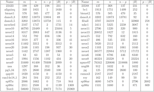
AAP lp: Derived from BCP lp user, this class contains the callbacks related to solving the LP relaxations in each search tree node. In this section, we present computational results that demonstrate the relative performance of the black-box solvers reviewed in Section 4. A performance profile is a relative measure of the efficiency of a solver compared to a group of solversS on a set of problem instances P.
Hence, ρs(τ) is the fraction of cases for which the solver performance is within a factor of τ of the best. The conclusions drawn here about the relative effectiveness of the MILP solvers should be considered with these caveats in mind. The graph shows that bonsaiG and MINTO were able to solve the largest fraction of the cases the fastest.
In Figure 6, we give the performance profile of the six MILP solvers on the cases where no solver was able to prove the optimality of the solution. Implementing a state-of-the-art primal heuristic in a non-commercial code would be a significant contribution. Looking ahead, we see no slowing down of the current trend of developing competitive non-commercial software for solving MILPs.