Classification of demand profiles based on booking data for the tourism sector

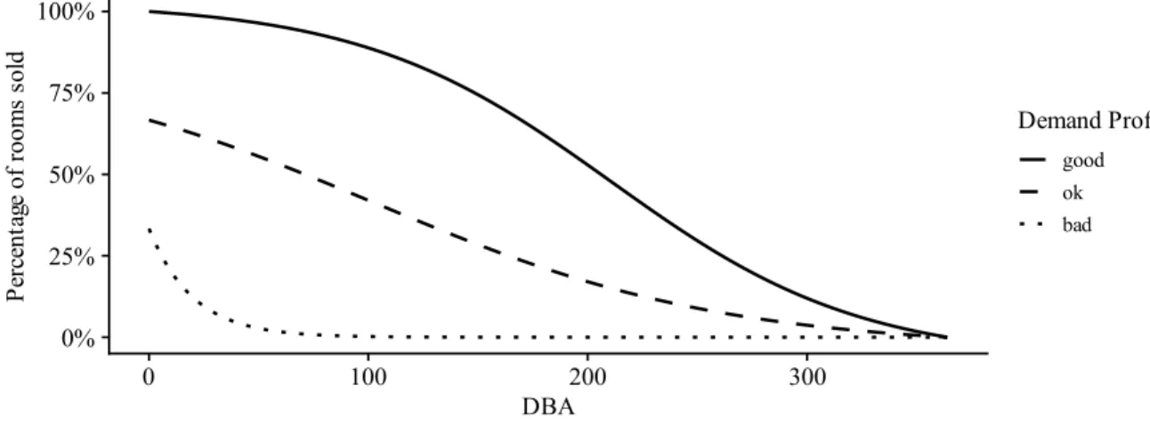
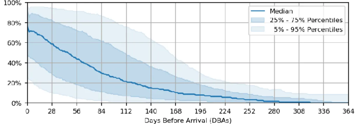
Distribution of income across DBAs for all 5 demand profiles in the selected set generated using quantile rules. Distribution of income across DBAs for all 5 demand profiles in the selected set generated using the Euclidean distance measure with the Gaussian mixture.

Introduction

In section 4 we present our methodology, defining each stage between the extraction of the data from the hotel data sources and the prediction of the demand profiles for future stay dates. In part 5, we present a use case of our methodology, using a real-world hotel as an example.

Background

Revenue management & Hospitality

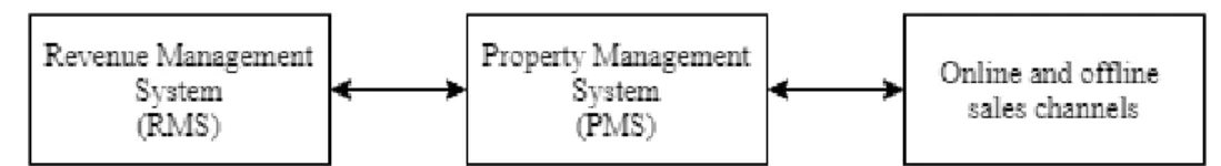
The consolidation of these free markets and the advent of the Internet have led to the increasing importance of solid revenue management. As you can see in Fig 3, the number of companies selling RMSs has exploded in the last 30 years.

Seasonality

Natural factors – related to the regular and recurring temporal variations in the natural phenomena, especially those related to the climate and the seasons of the year. The institutional factors can be push factors when it comes to holidays and vacations, or pull factors when it comes to special events and festivals in the destination country.

Literature Review

Tourism and hospitality

20, where 𝑑𝑖 is the local trend for a particular point in time, 𝑙𝑖 is the local level following a random walk, 𝑠𝑖 is the influence of the season for each particular point in time with a cycle of length 𝑛𝑠 and 𝜖𝑖 is white noise following a normal distribution. Another interesting forecasting methodology with information retrieval capabilities is the use of binary period variables (quarterly, monthly, weekly, .

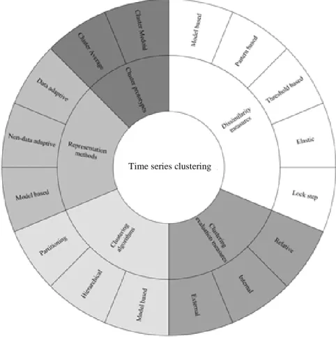
Time series clustering

• Representation methods
• Dissimilarity measures
• Clustering algorithms
• Cluster prototypes
• Clustering evaluation measures

Model-Based Measures – This type of difference measure uses a completely different approach to comparing time series. Given time series 𝑇 and 𝑄 with lengths 𝑛 and 𝑚, respectively, the distance matrix 𝑛 × 𝑚 is the matrix 𝑀, where 𝑀𝑖,𝑗= 𝑑(𝑡𝑖, 𝑞𝑗).

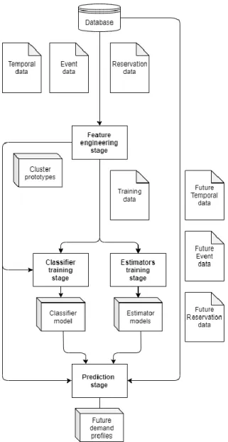
Methodology

• Feature engineering stage
• Data wrangling phase
• Demand profile labelling phase
• Classifier training stage
• Pessimistic strategy
• Optimistic strategy
• Estimators training stage
• Additive Pickup method
• Traditional regression
• Recurrent Neural Networks
• Prediction stage

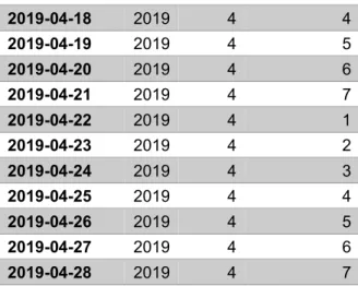
In the classifier training stage, we will train a classifier to predict the demand profile for a given stay date. Booking DBA (number) – the number of days before the day of stay on which the booking was booked. Cancellation DBA (number) – the number of days before the stay date on which the stay date of the reservation was cancelled.

As an example, based on the reservation data presented in Table 4, we calculated the reservation curves for both the rooms and revenue for the stay date of in Table 6. The demand profile data was compiled from the correspondence between each stay date analyzed and its group ID as the demand profile (as presented in Table 8). The residence date, month and day of the week are static attributes, as they are fully observable.

This is another way to study the problem that estimators are solving, based on the booking curve data from the training data, we can transform the data for each stay date as a sequence of rooms sold and revenue generated in the days before the stay date. The calendar data is then fed into a pessimistic classifier as training data to classify the demand profile for each stay date.

Case Study

Feature Engineering stage

• Data Wrangling phase
• Demand profile labelling phase

The best number of demand profiles is then selected from the value in the corner of the RMSE curve. Based on the measure we defined at the beginning of this section, the score for sets of demand profiles generated from the k-means clustering algorithm ranged between 5.491% and 4.401%, with the best number of demand profiles being 5 with a score of 4.653. %. The score for sets of demand profiles generated from the Gaussian mixture clustering algorithm ranged between 5.491% and 4.346%, and the best number of demand profiles was again 5 with a score of 4.641%.

Distribution of sales among DBAs for all five demand profiles in the selected set, generated using the LB_Keogh distance measure with the k-medoids. With the modified measure, the score for the question profile sets generated using the cross-correlation distance with a maximum radius of 0 ranged between 5.686% and 5.206%, and the best number of question profiles was 6 with a score of 5.295%. The score for the question profile sets generated using the cross-correlation distance with a maximum radius of 7 ranged between 5.674% and 5.201%, and the best number of question profiles was 6 with a score of 5.284%.

Classifier training stage

For the optimistic classifiers, we used all calendar data, booking curve data and cluster data as a set of independent variables to classify the demand profile for the different stay dates. Specifically for the cluster data, the cluster prototype for each demand profile was extracted from the cluster analysis performed in the demand profile labeling phase from the previous step. For each stay date in the booking curve data, we measured the distance from it to the cluster prototype for each demand profile and added it to the training data.

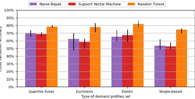
59 As before, for each pair of classification algorithms and demand profile set, we trained 5 different models on different stay dates and tested their accuracy with stay dates left out of the training data. The classification algorithm showing the best accuracy over all types of demand profile sets was the random forest classifier, with an average accuracy of and 90.471% for quantile rules, Euclidean, elastic and based demand profile sets shape respectively. The minimum, average, and maximum accuracy for all pairs of classification algorithm and demand profile group type is shown in Fig. 28.

Estimator training stage

The RMSE values ​​for the final number of rooms sold and revenue earned, from 0 to 12 months from the date of stay are shown in Figs 29 and 30 respectively. With this linear regression, the RMSE values ​​for the final number of rooms sold ranged between 2.715%. The RMSE values ​​for the final number of rooms sold and revenue earned, from 0 to 12 months from the stay date are shown in Figs 29 and 30, respectively, for both linear regression and random forest.

RMSE of the last rooms sold from 0 to 12 months to the stay date for all estimators. RMSE of final income obtained from 0 to 12 months to the residency date for all estimators. We also tried to train a sequential estimator with a recurrent neural network but failed. In the first scenario, which was the best, the model would give somewhat good results up to 1 week to the stay date.

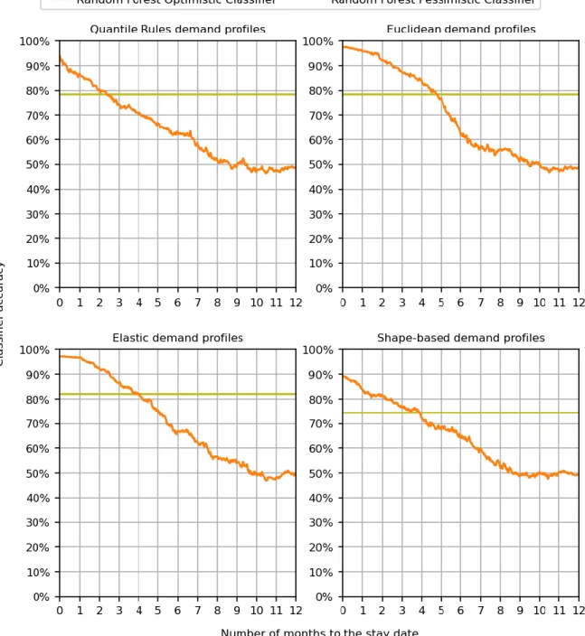
Prediction stage

It is common to see that the predicted demand profiles that are false negatives are usually classified as the previous or the next demand profile. This means that even when the classifier does not correctly classify the demand profile of a stay date, it is not far from the true demand profile. Accuracy for all demand profile types, from 0 to 12 months to the occupancy date, using the random forest classifiers and random forest estimators.

Critical Analysis

Looking at the demand profile set selected by the scoring function in section 5.1.2, the demand profiles between them are quite similar. What we are talking about here can be easily seen in the demand profiles in section 5.1.2, if we compare the empirical income distribution of the demand profiles produced by quantile rules with the demand profiles produced by the elastic or Euclidean measures. Considering the amendments in the last DBAs closer to the residency date, this is to be expected.

Finally, the Euclidean and elastic demand profiles performed better, while the elastic demand profiles performed the best of the two. On the other hand, the minimum percentage of true positives in the elastic demand profiles was seen in the real demand profile 3 with 26.087% of the representation. However, when we compare the demand profiles from Figures 22 and 24 in section 5.1.2 for the Euclidean and elastic demand profiles, we see that there is a better separation between the elastic demand profiles, compared to the Euclidean demand profiles, which we believe is one of the main reasons for the difference in classification performance.

Conclusion

Future work

An investigation of this methodology using more data (at least 3 years) would allow the use of LSTM or GRU recurrent neural networks as both an optimistic classifier and an estimator. A test that could be done would be that instead of having separate models for estimation and classification, we could have a single recurrent neural network that would integrate both, using padding on the time series when the characteristics of certain DBAs were not observable. We could also get more information from the classifiers we trained about which features have the most influence on each demand profile, using feature importance or methods such as SHapley Additive exPlanations (SHAP).

With this information, hotel managers could better understand what defines each demand profile and could actively influence market demand to bring dates of stay into a higher demand profile. Another extension of the methodology we developed would be to include or better handle market segmentation data in the demand profiles. However, these would be two completely different situations, where the first case could be a stay date with a lower demand profile than the second case, although similar in the way we look at it.

Keogh, EJ, Pazzani, MJ: An improved time series representation enabling fast and accurate classification, clustering and relevance feedback. Keogh, E.J., Pazzani, M.J.: A simple dimensionality reduction technique for fast similarity searching in large time series databases. Wang,

Bagnall, A., Lines, J., Bostrom, A., Large, J., Keogh, E.: The amazing time series classification bake off: a review and experimental evaluation of recent algorithmic advances. Hewamalage, H., Bergmeir, C., Bandara, K.: Recurrent neural networks for time series forecasting: current status and future directions. Möller-Levet, C.S., Klawonn, F., Cho, K.-H., Wolkenhauer, O.: Fuzzy Clustering of Short Time- Series and Unevenly Distributed Sampling Points BT - Advances in Intelligent Data Analysis V.