2550 Garcia Avenue Mountain View, CA 94043 U.S.A.
What Every Computer Scientist Should Know About Floating-Point Arithmetic
Part No: 800-7895-10 Revision A, June 1992
1994 Sun Microsystems, Inc.
2550 Garcia Avenue, Mountain View, California 94043-1100 U.S.A.
All rights reserved. This product and related documentation are protected by copyright and distributed under licenses restricting its use, copying, distribution, and decompilation. No part of this product or related documentation may be reproduced in any form by any means without prior written authorization of Sun and its licensors, if any.
Portions of this product may be derived from the UNIX® and Berkeley 4.3 BSD systems, licensed from UNIX System Laboratories, Inc., a wholly owned subsidiary of Novell, Inc., and the University of California, respectively. Third-party font software in this product is protected by copyright and licensed from Sun’s font suppliers.
RESTRICTED RIGHTS LEGEND: Use, duplication, or disclosure by the United States Government is subject to the restrictions set forth in DFARS 252.227-7013 (c)(1)(ii) and FAR 52.227-19.
The product described in this manual may be protected by one or more U.S. patents, foreign patents, or pending applications.
TRADEMARKS
Sun, the Sun logo, Sun Microsystems, Sun Microsystems Computer Corporation, Solaris, are trademarks or registered trademarks of Sun Microsystems, Inc. in the U.S. and certain other countries. UNIX is a registered trademark of Novell, Inc., in the United States and other countries; X/Open Company, Ltd., is the exclusive licensor of such trademark. OPEN LOOK® is a registered trademark of Novell, Inc. PostScript and Display PostScript are trademarks of Adobe Systems, Inc. All other product names mentioned herein are the trademarks of their respective owners.
All SPARC trademarks, including the SCD Compliant Logo, are trademarks or registered trademarks of SPARC International, Inc. SPARCstation, SPARCserver, SPARCengine, SPARCstorage, SPARCware, SPARCcenter, SPARCclassic, SPARCcluster, SPARCdesign, SPARC811, SPARCprinter, UltraSPARC, microSPARC, SPARCworks, and SPARCompiler are licensed exclusively to Sun Microsystems, Inc. Products bearing SPARC trademarks are based upon an architecture developed by Sun Microsystems, Inc.
The OPEN LOOKand Sun™ Graphical User Interfaces were developed by Sun Microsystems, Inc. for its users and licensees.
Sun acknowledges the pioneering efforts of Xerox in researching and developing the concept of visual or graphical user interfaces for the computer industry. Sun holds a non-exclusive license from Xerox to the Xerox Graphical User Interface, which license also covers Sun’s licensees who implement OPEN LOOK GUIs and otherwise comply with Sun’s written license agreements.
X Window System is a product of the Massachusetts Institute of Technology.
THIS PUBLICATION IS PROVIDED “AS IS” WITHOUT WARRANTY OF ANY KIND, EITHER EXPRESS OR IMPLIED, INCLUDING, BUT NOT LIMITED TO, THE IMPLIED WARRANTIES OF MERCHANTABILITY, FITNESS FOR A PARTICULAR PURPOSE, OR NON-INFRINGEMENT.
THIS PUBLICATION COULD INCLUDE TECHNICAL INACCURACIES OR TYPOGRAPHICAL ERRORS. CHANGES ARE PERIODICALLY ADDED TO THE INFORMATION HEREIN; THESE CHANGES WILL BE INCORPORATED IN NEW EDITIONS OF THE PUBLICATION. SUN MICROSYSTEMS, INC. MAY MAKE IMPROVEMENTS AND/OR CHANGES IN THE PRODUCT(S) AND/OR THE PROGRAM(S) DESCRIBED IN THIS PUBLICATION AT ANY TIME
Contents
Abstract . . . 1
Introduction . . . 2
Rounding Error . . . 2
Floating-point Formats . . . 3
Relative Error and Ulps . . . 5
Guard Digits . . . 6
Cancellation . . . 8
The IEEE Standard . . . 17
Formats and Operations . . . 18
Special Quantities . . . 24
NaNs. . . 25
Exceptions, Flags and Trap Handlers . . . 32
Systems Aspects . . . 37
Instruction Sets. . . 38
Languages and Compilers . . . 40
Exception Handling. . . 48
The Details . . . 50
Rounding Error . . . 50
Errors In Summation . . . 61
Summary. . . 62
Acknowledgments . . . 63
References . . . 63
Theorem 14 and Theorem 8 . . . 65
What Every Computer Scientist Should Know About Floating-Point Arithmetic
Note –This document is a reprint of the paper What Every Computer Scientist Should Know About Floating-Point Arithmetic, published in the March, 1991 issue of Computing Surveys. Copyright 1991, Association for Computing
Machinery, Inc., reprinted by permission.
Abstract
Floating-point arithmetic is considered an esoteric subject by many people.
This is rather surprising because floating-point is ubiquitous in computer systems. Almost every language has a floating-point datatype; computers from PC’s to supercomputers have floating-point accelerators; most compilers will be called upon to compile floating-point algorithms from time to time; and virtually every operating system must respond to floating-point exceptions such as overflow. This paper presents a tutorial on those aspects of floating- point that have a direct impact on designers of computer systems. It begins with background on floating-point representation and rounding error,
continues with a discussion of the IEEE floating-point standard, and concludes with numerous examples of how computer builders can better support floating-point.
Categories and Subject Descriptors: (Primary) C.0 [Computer Systems Organization]: General
—
instruction set design; D.3.4 [ProgrammingLanguages]: Processors
—
compilers, optimization; G.1.0 [Numerical Analysis]:General
—
computer arithmetic, error analysis, numerical algorithms (Secondary)D.2.1 [Software Engineering]: Requirements/Specifications
—
languages; D.3.4 [Programming Languages]: Formal Definitions and Theory—
semantics; D.4.1 [Operating Systems]: Process Management—
synchronization.General Terms: Algorithms, Design, Languages
Additional Key Words and Phrases: Denormalized number, exception, floating- point, floating-point standard, gradual underflow, guard digit, NaN, overflow, relative error, rounding error, rounding mode, ulp, underflow.
Introduction
Builders of computer systems often need information about floating-point arithmetic. There are, however, remarkably few sources of detailed information about it. One of the few books on the subject, Floating-Point Computation by Pat Sterbenz, is long out of print. This paper is a tutorial on those aspects of floating-point arithmetic (floating-point hereafter) that have a direct connection to systems building. It consists of three loosely connected parts. The first (Section , “Rounding Error,” on page 2) discusses the implications of using different rounding strategies for the basic operations of addition, subtraction, multiplication and division. It also contains background information on the two methods of measuring rounding error,ulps andrelative error. The second part discusses the IEEE floating-point standard, which is becoming rapidly accepted by commercial hardware manufacturers. Included in the IEEE standard is the rounding method for basic operations. The discussion of the standard draws on the material in Section , “Rounding Error,” on page 2. The third part discusses the connections between floating-point and the design of various aspects of computer systems. Topics include instruction set design, optimizing compilers and exception handling.
I have tried to avoid making statements about floating-point without also giving reasons why the statements are true, especially since the justifications involve nothing more complicated than elementary calculus. Those
explanations that are not central to the main argument have been grouped into a section called“The Details,” so that they can be skipped if desired. In particular, the proofs of many of the theorems appear in this section. The end of each proof is marked with the❚ symbol; when a proof is not included, the❚ appears immediately following the statement of the theorem.
Rounding Error
Squeezing infinitely many real numbers into a finite number of bits requires an approximate representation. Although there are infinitely many integers, in most programs the result of integer computations can be stored in 32 bits. In
contrast, given any fixed number of bits, most calculations with real numbers will produce quantities that cannot be exactly represented using that many bits. Therefore the result of a floating-point calculation must often be rounded in order to fit back into its finite representation. This rounding error is the characteristic feature of floating-point computation. “Relative Error and Ulps”
on page 5 describes how it is measured.
Since most floating-point calculations have rounding error anyway, does it matter if the basic arithmetic operations introduce a little bit more rounding error than necessary? That question is a main theme throughout this section.
“Guard Digits” on page 6 discusses guard digits, a means of reducing the error when subtracting two nearby numbers. Guard digits were considered
sufficiently important by IBM that in 1968 it added a guard digit to the double precision format in the System/360 architecture (single precision already had a guard digit), and retrofitted all existing machines in the field. Two examples are given to illustrate the utility of guard digits.
The IEEE standard goes further than just requiring the use of a guard digit. It gives an algorithm for addition, subtraction, multiplication, division and square root, and requires that implementations produce the same result as that algorithm. Thus when a program is moved from one machine to another, the results of the basic operations will be the same in every bit if both machines support the IEEE standard. This greatly simplifies the porting of programs.
Other uses of this precise specification are given in “Exactly Rounded Operations” on page 13.
Floating-point Formats
Several different representations of real numbers have been proposed, but by far the most widely used is the floating-point representation.1 Floating-point representations have a baseβ (which is always assumed to be even) and a precision p. Ifβ = 10 and p = 3 then the number 0.1 is represented as 1.00× 10⁻¹. Ifβ = 2 and p = 24, then the decimal number 0.1 cannot be represented exactly but is approximately 1.10011001100110011001101 × 2-4. In general, a floating- point number will be represented as±d.dd… d× βe, where d.dd… d is called the significand2and has p digits. More precisely±d0 . d1 d2…dp-1× βe represents the number
(1)
1. Examples of other representations are floating slash and signed logarithm [Matula and Kornerup 1985;
Swartzlander and Alexopoulos 1975].
2. This term was introduced by Forsythe and Moler [1967], and has generally replaced the older term mantissa.
d0+d1β−1+…+dp−1β−(p−1)
( ) βe,(0≤di<β)
±
The term floating-point number will be used to mean a real number that can be exactly represented in the format under discussion. Two other parameters associated with floating-point representations are the largest and smallest allowable exponents, emax and emin. Since there areβp possible significands, and emax - emin + 1 possible exponents, a floating-point number can be encoded in
bits, where the final +1 is for the sign bit. The precise encoding is not important for now.
There are two reasons why a real number might not be exactly representable as a floating-point number. The most common situation is illustrated by the decimal number 0.1. Although it has a finite decimal representation, in binary it has an infinite repeating representation. Thus whenβ = 2, the number 0.1 lies strictly between two floating-point numbers and is exactly representable by neither of them. A less common situation is that a real number is out of range, that is, its absolute value is larger thanβ × βemax or smaller than 1.0× βemin. Most of this paper discusses issues due to the first reason. However, numbers that are out of range will be discussed in “Infinity” on page 27 and
“Denormalized Numbers” on page 29.
Floating-point representations are not necessarily unique. For example, both 0.01× 101 and 1.00× 10⁻¹ represent 0.1. If the leading digit is nonzero (d0≠ 0 in equation (1) above), then the representation is said to be normalized. The floating-point number 1.00× 10⁻¹ is normalized, while 0.01× 101 is not. When β= 2, p = 3, emin = -1 and emax = 2 there are 16 normalized floating-point numbers, as shown in Figure 1. The bold hash marks correspond to numbers whose significand is 1.00. Requiring that a floating-point representation be normalized makes the representation unique. Unfortunately, this restriction makes it impossible to represent zero! A natural way to represent 0 is with 1.0× βemin-1, since this preserves the fact that the numerical ordering of nonnegative real numbers corresponds to the lexicographic ordering of their floating-point representations.3 When the exponent is stored in a k bit field, that means that only 2k - 1 values are available for use as exponents, since one must be reserved to represent 0.
Note that the× in a floating-point number is part of the notation, and different from a floating-point multiply operation. The meaning of the× symbol should be clear from the context. For example, the expression (2.5× 10-3)× (4.0× 102) involves only a single floating-point multiplication.
3. This assumes the usual arrangement where the exponent is stored to the left of the significand.
log2(emax−emin+1) + log2( )βp +1
Figure 1 Normalized numbers whenβ = 2, p = 3, emin = -1, emax = 2
Relative Error and Ulps
Since rounding error is inherent in floating-point computation, it is important to have a way to measure this error. Consider the floating-point format with β= 10 and p = 3, which will be used throughout this section. If the result of a floating-point computation is 3.12× 10⁻², and the answer when computed to infinite precision is .0314, it is clear that this is in error by 2 units in the last place. Similarly, if the real number .0314159 is represented as 3.14× 10⁻², then it is in error by .159 units in the last place. In general, if the floating-point number d.d…d× βe is used to represent z, then it is in error byd.d…d - (z/βe)βp-1units in the last place.4, 5The termulps will be used as shorthand for “units in the last place.” If the result of a calculation is the floating-point number nearest to the correct result, it still might be in error by as much as .5 ulp. Another way to measure the difference between a floating-point number and the real number it is approximating is relative error, which is simply the difference between the two numbers divided by the real number. For example the relative error committed when approximating 3.14159 by 3.14× 100 is .00159/3.14159≈ .0005.
To compute the relative error that corresponds to .5ulp, observe that when a real number is approximated by the closest possible floating-point number d.dd...dd × βe, the error can be as large as 0.00...00β′ × βe, whereβ’ is the digit β/2, there are p units in the significand of the floating point number, and p units of 0 in the significand of the error. This error is ((β/2)β-p)× βe. Since numbers of the form d.dd…dd× βe all have the same absolute error, but have values that range betweenβe andβ × βe, the relative error ranges between ((β/2)β-p) × βe/βe and ((β/2)β-p) × βe/βe+1. That is,
(2)
4. Unless the number z is larger thanβemax+1 or smaller thanβemin. Numbers which are out of range in this fashion will not be considered until further notice.
5. Let z’ be the floating point number that approximates z. Thend.d…d - (z/βe)βp-1 is equivalent to
z’-z/ulp(z’). (See Numerical Computation Guide for the definition of ulp(z)). A more accurate formula for measuring error isz’-z/ulp(z). -- Ed.
0 1 2 3 4 5 6 7
1 2β−p 1
2ulp β 2β−p
≤
≤
In particular, the relative error corresponding to .5 ulp can vary by a factor of β. This factor is called the wobble.Settingε = (β/2)β-p to the largest of the bounds in (2) above, we can say that when a real number is rounded to the closest floating-point number, the relative error is always bounded byε, which is referred to as machine epsilon.
In the example above, the relative error was .00159/3.14159≈ .0005. In order to avoid such small numbers, the relative error is normally written as a factor timesε, which in this case isε = (β/2)β-p = 5(10)-3 = .005. Thus the relative error would be expressed as (.00159/3.14159)/.005)ε ≈ 0.1ε.
To illustrate the difference between ulps and relative error, consider the real number x = 12.35. It is approximated by = 1.24 × 101. The error is 0.5ulps, the relative error is 0.8ε. Next consider the computation 8 . The exact value is 8x = 98.8, while the computed value is 8 = 9.92× 101. The error is now 4.0 ulps, but the relative error is still 0.8ε. The error measured inulps is 8 times larger, even though the relative error is the same. In general, when the base is β, a fixed relative error expressed inulps can wobble by a factor of up toβ.
And conversely, as equation (2) above shows, a fixed error of .5ulps results in a relative error that can wobble byβ.
The most natural way to measure rounding error is inulps. For example rounding to the nearest floating-point number corresponds to an error of less than or equal to .5ulp. However, when analyzing the rounding error caused by various formulas, relative error is a better measure. A good illustration of this is the analysis on page 51. Sinceε can overestimate the effect of rounding to the nearest floating-point number by the wobble factor ofβ, error estimates of formulas will be tighter on machines with a smallβ.
When only the order of magnitude of rounding error is of interest,ulps andε may be used interchangeably, since they differ by at most a factor ofβ. For example, when a floating-point number is in error by nulps, that means that the number of contaminated digits is logβ n. If the relative error in a
computation is nε, then
contaminated digits≈ logβ n. (3)
Guard Digits
One method of computing the difference between two floating-point numbers is to compute the difference exactly and then round it to the nearest floating- point number. This is very expensive if the operands differ greatly in size.
Assuming p = 3, 2.15× 10¹² - 1.25× 10⁻⁵ would be calculated as x˜
x˜
x˜
x = 2.15 × 10¹²
y = .0000000000000000125 × 1012 x - y = 2.1499999999999999875× 10¹²
which rounds to 2.15× 10¹². Rather than using all these digits, floating-point hardware normally operates on a fixed number of digits. Suppose that the number of digits kept is p, and that when the smaller operand is shifted right, digits are simply discarded (as opposed to rounding). Then
2.15×10¹²- 1.25×10⁻⁵ becomes x = 2.15 × 10¹²
y = 0.00 × 10¹² x - y = 2.15 × 10¹²
The answer is exactly the same as if the difference had been computed exactly and then rounded. Take another example: 10.1 - 9.93. This becomes
x = 1.01× 101 y = 0.99× 101 x - y = .02× 101
The correct answer is .17, so the computed difference is off by 30ulps and is wrong in every digit! How bad can the error be?
Theorem 1
Using a floating-point format with parametersβ and p, and computing differences using p digits, the relative error of the result can be as large asβ - 1.
Proof
A relative error ofβ - 1 in the expression x - y occurs when x = 1.00…0 and y =.ρρ…ρ, whereρ =β - 1. Here y has p digits (all equal toρ). The exact difference is x - y =β-p. However, when computing the answer using only p digits, the rightmost digit of y gets shifted off, and so the computed
difference isβ-p+1. Thus the error isβ-p -β-p+1 =β-p (β - 1), and the relative error isβ-p(β - 1)/β-p =β - 1.❚
Whenβ=2, the relative error can be as large as the result, and whenβ=10, it can be 9 times larger. Or to put it another way, whenβ=2, equation (3) above shows that the number of contaminated digits is log2(1/ε) = log2(2p) = p. That is, all of the p digits in the result are wrong! Suppose that one extra digit is added to guard against this situation (a guard digit). That is, the smaller number is truncated to p + 1 digits, and then the result of the subtraction is rounded to p digits. With a guard digit, the previous example becomes
x = 1.010 × 101 y = 0.993 × 101 x - y = .017× 101
and the answer is exact. With a single guard digit, the relative error of the result may be greater thanε, as in 110 - 8.59.
x = 1.10 × 10² y = .085× 102 x - y = 1.015× 10²
This rounds to 102, compared with the correct answer of 101.41, for a relative error of .006, which is greater thanε = .005. In general, the relative error of the result can be only slightly larger thanε. More precisely,
Theorem 2
If x and y are floating-point numbers in a format with parametersβ and p, and if subtraction is done with p + 1 digits (i.e. one guard digit), then the relative rounding error in the result is less than 2ε.
This theorem will be proven in “Rounding Error” on page 50. Addition is included in the above theorem since x and y can be positive or negative.
Cancellation
The last section can be summarized by saying that without a guard digit, the relative error committed when subtracting two nearby quantities can be very large. In other words, the evaluation of any expression containing a subtraction (or an addition of quantities with opposite signs) could result in a relative error so large that all the digits are meaningless (Theorem 1). When subtracting nearby quantities, the most significant digits in the operands match and cancel each other. There are two kinds of cancellation: catastrophic and benign.
Catastrophic cancellation occurs when the operands are subject to rounding errors. For example in the quadratic formula, the expression b2 - 4ac occurs.
The quantities b2 and 4ac are subject to rounding errors since they are the results of floating-point multiplications. Suppose that they are rounded to the nearest floating-point number, and so are accurate to within .5ulp. When they are subtracted, cancellation can cause many of the accurate digits to disappear, leaving behind mainly digits contaminated by rounding error. Hence the difference might have an error of many ulps. For example, consider b = 3.34, a = 1.22, and c = 2.28. The exact value of b2 - 4ac is .0292. But b2 rounds to 11.2 and 4ac rounds to 11.1, hence the final answer is .1 which is an error by 70
ulps, even though 11.2 - 11.1 is exactly equal to .16. The subtraction did not introduce any error, but rather exposed the error introduced in the earlier multiplications.
Benign cancellation occurs when subtracting exactly known quantities. If x and y have no rounding error, then by Theorem 2 if the subtraction is done with a guard digit, the difference x-y has a very small relative error (less than 2ε).
A formula that exhibits catastrophic cancellation can sometimes be rearranged to eliminate the problem. Again consider the quadratic formula
(4)
When , then does not involve a cancellation and .
But the other addition (subtraction) in one of the formulas will have a catastrophic cancellation. To avoid this, multiply the numerator and denominator of r1 by
(and similarly for r2) to obtain
(5)
If and , then computing r1 using formula (4) will involve a cancellation. Therefore, use (5) for computing r1 and (4) for r2. On the other hand, if b < 0, use (4) for computing r1 and (5) for r2.
The expression x2 - y2 is another formula that exhibits catastrophic cancellation.
It is more accurate to evaluate it as (x - y)(x + y).7 Unlike the quadratic formula, this improved form still has a subtraction, but it is a benign cancellation of quantities without rounding error, not a catastrophic one. By Theorem 2, the
6. 700, not 70. Since .1 - .0292 = .0708, the error in terms of ulp(0.0292) is 708 ulps. -- Ed.
r1 −b+ b2−4ac
2a ,r2 −b− b2−4ac
= = 2a
b2»ac b2−4ac b2−4ac≈ b
−b− b2−4ac
r1 2c
−b− b2−4ac r2
, 2c
−b+ b2−4ac
= =
b2»ac b>0
relative error in x - y is at most 2ε. The same is true of x + y. Multiplying two quantities with a small relative error results in a product with a small relative error (see “Rounding Error” on page 50).
In order to avoid confusion between exact and computed values, the following notation is used. Whereas x - y denotes the exact difference of x and y, x y denotes the computed difference (i.e., with rounding error). Similarly⊕,⊗, and
denote computed addition, multiplication, and division, respectively. All caps indicate the computed value of a function, as in LN(x) or SQRT(x). Lower case functions and traditional mathematical notation denote their exact values as in ln(x) and .
Although (x y)⊗ (x⊕y) is an excellent approximation to x2 - y2, the floating-point numbers x and y might themselves be approximations to some true quantities and . For example, and might be exactly known decimal numbers that cannot be expressed exactly in binary. In this case, even though x y is a good approximation to x - y, it can have a huge relative error compared to the true expression , and so the advantage of (x + y)(x - y) over x2 - y2 is not as dramatic. Since computing (x + y)(x - y) is about the same amount of work as computing x2 - y2, it is clearly the preferred form in this case. In general, however, replacing a catastrophic cancellation by a benign one is not worthwhile if the expense is large because the input is often (but not always) an approximation. But eliminating a cancellation entirely (as in the quadratic formula) is worthwhile even if the data are not exact. Throughout this paper, it will be assumed that the floating-point inputs to an algorithm are exact and that the results are computed as accurately as possible.
The expression x2 - y2 is more accurate when rewritten as (x - y)(x + y) because a catastrophic cancellation is replaced with a benign one. We next present more interesting examples of formulas exhibiting catastrophic cancellation that can be rewritten to exhibit only benign cancellation.
The area of a triangle can be expressed directly in terms of the lengths of its sides a, b, and c as
(6)
7. Although the expression (x - y)(x + y) does not cause a catastrophic cancellation, it is slightly less accurate than x2 - y2 if or . In this case, (x - y)(x + y) has three rounding errors, but x2 - y2 has only two since the rounding error committed when computing the smaller of x2 and y2 does not affect the final subtraction.
x y» x y« x
xˆ yˆ xˆ yˆ
xˆ−yˆ
A = s s( −a) (s−b)(s−c),where s = (a+ +b c) ⁄2
Suppose the triangle is very flat; that is, a≈b + c. Then s≈a, and the term (s - a) in eq. (6) subtracts two nearby numbers, one of which may have rounding error. For example, if a = 9.0, b = c = 4.53, then the correct value of s is 9.03 and A is 2.342... . Even though the computed value of s (9.05) is in error by only 2 ulps, the computed value of A is 3.04, an error of 70ulps.
There is a way to rewrite formula (6) so that it will return accurate results even for flat triangles [Kahan 1986]. It is
(7) If a, b and c do not satisfy a ≥b≥c, simply rename them before applying (7). It is straightforward to check that the right-hand sides of (6) and (7) are
algebraically identical. Using the values of a, b, and c above gives a computed area of 2.35, which is 1ulp in error and much more accurate than the first formula.
Although formula (7) is much more accurate than (6) for this example, it would be nice to know how well (7) performs in general.
Theorem 3
The rounding error incurred when using (7) to compute the area of a triangle is at most 11ε, provided that subtraction is performed with a guard digit, e≤.005, and that square roots are computed to within 1/2ulp.
The condition that e < .005 is met in virtually every actual floating-point system. For example whenβ = 2, p≥ 8 ensures that e < .005, and whenβ = 10, p≥3 is enough.
In statements like Theorem 3 that discuss the relative error of an expression, it is understood that the expression is computed using floating-point arithmetic.
In particular, the relative error is actually of the expression
SQRT((a⊕ (b⊕c))⊗ (c (a b))⊗ (c⊕(a b))⊗ (a⊕(b c))) 4 (8)
Because of the cumbersome nature of (8), in the statement of theorems we will usually say the computed value of E rather than writing out E with circle notation.
A (a+ (b+c)) (c− (a−b)) (c+ (a−b)) (a+ (b−c))
4 ,a≥ ≥b c
=
Error bounds are usually too pessimistic. In the numerical example given above, the computed value of (7) is 2.35, compared with a true value of 2.34216 for a relative error of 0.7ε, which is much less than 11ε. The main reason for computing error bounds is not to get precise bounds but rather to verify that the formula does not contain numerical problems.
A final example of an expression that can be rewritten to use benign cancellation is (1 + x)n, where . This expression arises in financial calculations. Consider depositing $100 every day into a bank account that earns an annual interest rate of 6%, compounded daily. If n = 365 and i = .06, the amount of money accumulated at the end of one year is 100
dollars. If this is computed usingβ = 2 and p = 24, the result is $37615.45 compared to the exact answer of $37614.05, a discrepancy of $1.40. The reason for the problem is easy to see. The expression 1 + i/n involves adding 1 to .0001643836, so the low order bits of i/n are lost. This rounding error is amplified when 1 + i/n is raised to the nth power.
The troublesome expression (1 + i/n)n can be rewritten as enln(1 + i/n), where now the problem is to compute ln(1 + x) for small x. One approach is to use the approximation ln(1 + x)≈x, in which case the payment becomes $37617.26, which is off by $3.21 and even less accurate than the obvious formula. But there is a way to compute ln(1 + x) very accurately, as Theorem 4 shows [Hewlett-Packard 1982]. This formula yields $37614.07, accurate to within two cents!
Theorem 4 assumes that LN (x) approximates ln(x) to within 1/2ulp. The problem it solves is that when x is small, LN(1⊕x) is not close to ln(1 + x) because 1⊕x has lost the information in the low order bits of x. That is, the computed value of ln(1 + x) is not close to its actual value when . Theorem 4
If ln(1 + x) is computed using the formula
x for 1⊕x = 1ln(1 + x) =
for 1⊕x ≠ 1the relative error is at most 5ε when 0≤ x < , provided subtraction is performed with a guard digit, e < 0.1, and ln is computed to within 1/2ulp.
x 1«
1+i n⁄ ( )n−1
i n⁄
x 1«
x ln(1+x) 1+x ( ) −1
3 4
This formula will work for any value of x but is only interesting for , which is where catastrophic cancellation occurs in the naive formula ln(1 + x).
Although the formula may seem mysterious, there is a simple explanation for why it works. Write ln(1 + x) as . The left hand factor can be computed exactly, but the right hand factorµ(x) = ln(1 + x)/x will suffer a large rounding error when adding 1 to x. However,µ is almost constant, since ln(1 + x)≈x. So changing x slightly will not introduce much error. In other words, if , computing will be a good approximation to xµ(x)
= ln(1 + x). Is there a value for for which and can be computed accurately? There is; namely = (1⊕ x) 1, because then 1 + is exactly equal to 1⊕x.
The results of this section can be summarized by saying that a guard digit guarantees accuracy when nearby precisely known quantities are subtracted (benign cancellation). Sometimes a formula that gives inaccurate results can be rewritten to have much higher numerical accuracy by using benign
cancellation; however, the procedure only works if subtraction is performed using a guard digit. The price of a guard digit is not high, because it merely requires making the adder one bit wider. For a 54 bit double precision adder, the additional cost is less than 2%. For this price, you gain the ability to run many algorithms such as the formula (6) for computing the area of a triangle and the expression ln(1 + x). Although most modern computers have a guard digit, there are a few (such as Crays) that do not.
Exactly Rounded Operations
When floating-point operations are done with a guard digit, they are not as accurate as if they were computed exactly then rounded to the nearest floating- point number. Operations performed in this manner will be called exactly rounded.8 The example immediately preceding Theorem 2 shows that a single guard digit will not always give exactly rounded results. The previous section gave several examples of algorithms that require a guard digit in order to work properly. This section gives examples of algorithms that require exact
rounding.
So far, the definition of rounding has not been given. Rounding is straightforward, with the exception of how to round halfway cases; for example, should 12.5 round to 12 or 13? One school of thought divides the 10 digits in half, letting {0, 1, 2, 3, 4} round down, and {5, 6, 7, 8, 9} round up; thus
8. Also commonly referred to as correctly rounded. -- Ed.
x 1«
x ln(1+x)
( x ) = xµ( )x
x˜≈x xµ( )x˜
x˜ x˜ x˜+1
x˜ x˜
12.5 would round to 13. This is how rounding works on Digital Equipment Corporation’s VAX™ computers. Another school of thought says that since numbers ending in 5 are halfway between two possible roundings, they should round down half the time and round up the other half. One way of obtaining this 50% behavior to require that the rounded result have its least significant digit be even. Thus 12.5 rounds to 12 rather than 13 because 2 is even. Which of these methods is best, round up or round to even? Reiser and Knuth [1975]
offer the following reason for preferring round to even.
Theorem 5
Let x and y be floating-point numbers, and define x0 = x, x1 = (x0 y)⊕ y,…, xn= (xn-1 y)⊕ y. If⊕ and are exactly rounded using round to even, then either xn = x for all n or xn = x1 for all n≥ 1.❚
To clarify this result, considerβ = 10, p = 3 and let x = 1.00, y = -.555. When rounding up, the sequence becomes x0 y = 1.56, x1 = 1.56 .555 = 1.01, x1 y = 1.01⊕ .555 = 1.57, and each successive value of xn increases by .01, until xn = 9.45 (n≤ 845)9 Under round to even, xn is always 1.00. This example suggests that when using the round up rule, computations can gradually drift upward, whereas when using round to even the theorem says this cannot happen. Throughout the rest of this paper, round to even will be used.
One application of exact rounding occurs in multiple precision arithmetic.
There are two basic approaches to higher precision. One approach represents floating-point numbers using a very large significand, which is stored in an array of words, and codes the routines for manipulating these numbers in assembly language. The second approach represents higher precision floating- point numbers as an array of ordinary floating-point numbers, where adding the elements of the array in infinite precision recovers the high precision floating-point number. It is this second approach that will be discussed here.
The advantage of using an array of floating-point numbers is that it can be coded portably in a high level language, but it requires exactly rounded arithmetic.
The key to multiplication in this system is representing a product xy as a sum, where each summand has the same precision as x and y. This can be done by splitting x and y. Writing x = xh + xl and y = yh + yl, the exact product is xy = xhyh + xhyl + xlyh + xlyl. If x and y have p bit significands, the summands will also have p bit significands provided that xl, xh, yh, yl can be represented using
p/2 bits. When p is even, it is easy to find a splitting. The number x0.x1…xp - 1 can be written as the sum of x0.x1…xp/2 - 1 and
9. When n = 845, xn= 9.45, xn + 0.555 = 10.0, and 10.0 - 0.555 = 9.45. Therefore, xn = x845 for n > 845.
0.0… 0xp/2…xp - 1. When p is odd, this simple splitting method won’t work.
An extra bit can, however, be gained by using negative numbers. For example, ifβ = 2, p = 5, and x = .10111, x can be split as xh = .11 and xl= -.00001. There is more than one way to split a number. A splitting method that is easy to compute is due to Dekker [1971], but it requires more than a single guard digit.
Theorem 6
Let p be the floating-point precision, with the restriction that p is even whenβ> 2, and assume that floating-point operations are exactly rounded. Then if k =p/2 is half the precision (rounded up) and m =βk + 1, x can be split as x = xh + xl, where xh = (m⊗ x) (m⊗ x x), xl = x xh, and each xi is representable using p/2
bits of precision.
To see how this theorem works in an example, letβ = 10, p = 4, b = 3.476, a = 3.463, and c = 3.479. Then b2 - ac rounded to the nearest floating-point number is .03480, while b⊗ b = 12.08, a⊗c = 12.05, and so the computed value of b2 - ac is .03. This is an error of 480ulps. Using Theorem 6 to write b = 3.5 - .024, a = 3.5 - .037, and c = 3.5 - .021, b2 becomes 3.52 - 2× 3.5× .024 + .0242. Each summand is exact, so b2 = 12.25 - .168 + .000576, where the sum is left
unevaluated at this point. Similarly, ac = 3.52 - (3.5× .037 + 3.5× .021) + .037× .021 = 12.25 - .2030 +.000777. Finally, subtracting these two series term by term gives an estimate for b2 - ac of 0⊕ .0350 .000201 = .03480, which is identical to the exactly rounded result. To show that Theorem 6 really requires exact rounding, consider p = 3,β = 2, and x = 7. Then m = 5, mx = 35, and m⊗x = 32.
If subtraction is performed with a single guard digit, then (m⊗x) x = 28.
Therefore, xh = 4 and xl = 3, hence xl is not representable withp/2 = 1 bit.
As a final example of exact rounding, consider dividing m by 10. The result is a floating-point number that will in general not be equal to m/10. Whenβ = 2, multiplying m/10 by 10 will miraculously restore m, provided exact rounding is being used. Actually, a more general fact (due to Kahan) is true. The proof is ingenious, but readers not interested in such details can skip ahead to Section ,
“The IEEE Standard,” on page 17.
Theorem 7
Whenβ = 2, if m and n are integers with |m| < 2p - 1 and n has the special form n
= 2i + 2j, then (m n)⊗ n = m, provided floating-point operations are exactly rounded.
Proof
Scaling by a power of two is harmless, since it changes only the exponent not the significand. If q = m/n, then scale n so that 2p - 1≤n < 2p and scale m so that < q < 1. Thus, 2p - 2 < m < 2p. Since m has p significant bits, it has at most one bit to the right of the binary point. Changing the sign of m is harmless, so assume that q > 0.
If = m n, to prove the theorem requires showing that
(9)
That is because m has at most 1 bit right of the binary point, so n will round to m. To deal with the halfway case when |n - m| = , note that since the initial unscaled m had |m| < 2p - 1, its low-order bit was 0, so the low-order bit of the scaled m is also 0. Thus, halfway cases will round to m.
Suppose that q = .q1q2…, and let = .q1q2…qp1. To estimate |n - m|, first compute | - q| = |N/2p + 1 - m/n|, where N is an odd integer. Since n = 2i+ 2j and 2p - 1≤n < 2p, it must be that n = 2p - 1 + 2k for some k≤p - 2, and thus
.
The numerator is an integer, and since N is odd, it is in fact an odd integer.
Thus, | - q|≥ 1/(n2p + 1 - k). Assume q < (the case q > is similar).10 Then n < m, and
|m-n | = m-n = n(q- ) = n(q-( -2-p-1) ) ≤
= (2p-1+2k)2-p-1+2-p-1+k =
This establishes (9) and proves the theorem11. ❚
10. Notice that in binary, q cannot equal . -- Ed.
11. Left as an exercise to the reader: extend the proof to bases other than 2. -- Ed.
1 2
q ⊕
nq−m 1
≤4
q
q 1
4
qˆ q
qˆ
qˆ−q nN−2p+1m n2p+1
2p−1−k+1
( )N−2p+1−km n2p+1−k
= =
qˆ qˆ qˆ
qˆ q
q q q qˆ n 2−p−1 1
n2p+1−k
−
1 4
The theorem holds true for any baseβ, as long as 2i + 2j is replaced byβi +βj. Asβ gets larger, however, denominators of the formβi +βj are farther and farther apart.
We are now in a position to answer the question, Does it matter if the basic arithmetic operations introduce a little more rounding error than necessary?
The answer is that it does matter, because accurate basic operations enable us to prove that formulas are “correct” in the sense they have a small relative error. “Cancellation” on page 8 discussed several algorithms that require guard digits to produce correct results in this sense. If the input to those formulas are numbers representing imprecise measurements, however, the bounds of Theorems 3 and 4 become less interesting. The reason is that the benign cancellation x - y can become catastrophic if x and y are only approximations to some measured quantity. But accurate operations are useful even in the face of inexact data, because they enable us to establish exact relationships like those discussed in Theorems 6 and 7. These are useful even if every floating-point variable is only an approximation to some actual value.
The IEEE Standard
There are two different IEEE standards for floating-point computation. IEEE 754 is a binary standard that requiresβ = 2, p = 24 for single precision and p = 53 for double precision [IEEE 1987]. It also specifies the precise layout of bits in a single and double precision. IEEE 854 allows eitherβ = 2 orβ = 10 and unlike 754, does not specify how floating-point numbers are encoded into bits [Cody et al. 1984]. It does not require a particular value for p, but instead it specifies constraints on the allowable values of p for single and double precision. The term IEEE Standard will be used when discussing properties common to both standards.
This section provides a tour of the IEEE standard. Each subsection discusses one aspect of the standard and why it was included. It is not the purpose of this paper to argue that the IEEE standard is the best possible floating-point standard but rather to accept the standard as given and provide an
introduction to its use. For full details consult the standards themselves [IEEE 1987; Cody et al. 1984].
Formats and Operations
Base
It is clear why IEEE 854 allowsβ = 10. Base ten is how humans exchange and think about numbers. Usingβ = 10 is especially appropriate for calculators, where the result of each operation is displayed by the calculator in decimal.
There are several reasons why IEEE 854 requires that if the base is not 10, it must be 2. “Relative Error and Ulps” on page 5 mentioned one reason: the results of error analyses are much tighter whenβ is 2 because a rounding error of .5ulp wobbles by a factor ofβ when computed as a relative error, and error analyses are almost always simpler when based on relative error. A related reason has to do with the effective precision for large bases. Considerβ = 16, p = 1 compared toβ = 2, p = 4. Both systems have 4 bits of significand.
Consider the computation of 15/8. Whenβ = 2, 15 is represented as 1.111× 23, and 15/8 as 1.111× 20. So 15/8 is exact. However, whenβ = 16, 15 is
represented as F× 160, where F is the hexadecimal digit for 15. But 15/8 is represented as 1× 160, which has only one bit correct. In general, base 16 can lose up to 3 bits, so that a precision of p hexidecimal digits can have an effective precision as low as 4p - 3 rather than 4p binary bits. Since large values ofβ have these problems, why did IBM chooseβ = 16 for its system/370? Only IBM knows for sure, but there are two possible reasons. The first is increased exponent range. Single precision on the system/370 hasβ = 16, p = 6. Hence the significand requires 24 bits. Since this must fit into 32 bits, this leaves 7 bits for the exponent and one for the sign bit. Thus the magnitude of representable numbers ranges from about to about = . To get a similar
exponent range whenβ = 2 would require 9 bits of exponent, leaving only 22 bits for the significand. However, it was just pointed out that whenβ = 16, the effective precision can be as low as 4p - 3 = 21 bits. Even worse, whenβ = 2 it is possible to gain an extra bit of precision (as explained later in this section), so theβ = 2 machine has 23 bits of precision to compare with a range of 21 – 24 bits for theβ = 16 machine.
Another possible explanation for choosingβ = 16 has to do with shifting. When adding two floating-point numbers, if their exponents are different, one of the significands will have to be shifted to make the radix points line up, slowing down the operation. In theβ = 16, p = 1 system, all the numbers between 1 and 15 have the same exponent, and so no shifting is required when adding any of the
(
152)
= 105 possible pairs of distinct numbers from this set. However, in the β = 2, p = 4 system, these numbers have exponents ranging from 0 to 3, and shifting is required for 70 of the 105 pairs.16−26 1626 228
In most modern hardware, the performance gained by avoiding a shift for a subset of operands is negligible, and so the small wobble ofβ = 2 makes it the preferable base. Another advantage of usingβ = 2 is that there is a way to gain an extra bit of significance.12 Since floating-point numbers are always
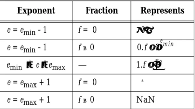
normalized, the most significant bit of the significand is always 1, and there is no reason to waste a bit of storage representing it. Formats that use this trick are said to have a hidden bit. It was already pointed out in “Floating-point Formats” on page 3 that this requires a special convention for 0. The method given there was that an exponent of emin - 1 and a significand of all zeros represents not , but rather 0.
IEEE 754 single precision is encoded in 32 bits using 1 bit for the sign, 8 bits for the exponent, and 23 bits for the significand. However, it uses a hidden bit, so the significand is 24 bits (p = 24), even though it is encoded using only 23 bits.
Precision
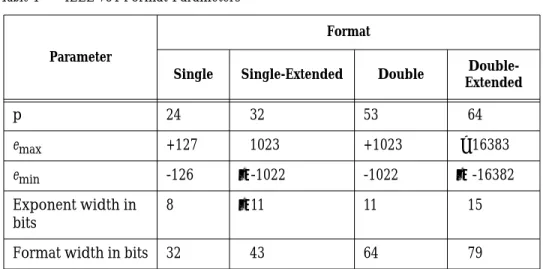
The IEEE standard defines four different precisions: single, double, single- extended, and double-extended. In 754, single and double precision correspond roughly to what most floating-point hardware provides. Single precision occupies a single 32 bit word, double precision two consecutive 32 bit words. Extended precision is a format that offers at least a little extra precision and exponent range (Table 1).
12. This appears to have first been published by Goldberg [1967], although Knuth ([ 1981], page 211) attributes this idea to Konrad Zuse.
1.0×2emin−1
The IEEE standard only specifies a lower bound on how many extra bits extended precision provides. The minimum allowable double-extended format is sometimes referred to as 80-bit format, even though the table shows it using 79 bits. The reason is that hardware implementations of extended precision normally don’t use a hidden bit, and so would use 80 rather than 79 bits.13 The standard puts the most emphasis on extended precision, making no recommendation concerning double precision, but strongly recommending that
Implementations should support the extended format corresponding to the widest basic format supported,…
One motivation for extended precision comes from calculators, which will often display 10 digits, but use 13 digits internally. By displaying only 10 of the 13 digits, the calculator appears to the user as a “black box” that computes exponentials, cosines, etc. to 10 digits of accuracy. For the calculator to compute functions like exp, log and cos to within 10 digits with reasonable efficiency, it needs a few extra digits to work with. It isn’t hard to find a simple rational expression that approximates log with an error of 500 units in the last
13. According to Kahan, extended precision has 64 bits of significand because that was the widest precision across which carry propagation could be done on the Intel 8087 without increasing the cycle time [Kahan 1988].
Table 1 IEEE 754 Format Parameters
Parameter
Format
Single Single-Extended Double Double- Extended
p 24 32 53 64
emax +127 1023 +1023 > 16383
emin -126 ≤ -1022 -1022 ≤ -16382
Exponent width in bits
8 ≤ 11 11 15
Format width in bits 32 43 64 79
place. Thus computing with 13 digits gives an answer correct to 10 digits. By keeping these extra 3 digits hidden, the calculator presents a simple model to the operator.
Extended precision in the IEEE standard serves a similar function. It enables libraries to efficiently compute quantities to within about .5ulp in single (or double) precision, giving the user of those libraries a simple model, namely that each primitive operation, be it a simple multiply or an invocation of log, returns a value accurate to within about .5ulp. However, when using extended precision, it is important to make sure that its use is transparent to the user. For example, on a calculator, if the internal representation of a displayed value is not rounded to the same precision as the display, then the result of further operations will depend on the hidden digits and appear unpredictable to the user.
To illustrate extended precision further, consider the problem of converting between IEEE 754 single precision and decimal. Ideally, single precision numbers will be printed with enough digits so that when the decimal number is read back in, the single precision number can be recovered. It turns out that 9 decimal digits are enough to recover a single precision binary number (see
“Binary to Decimal Conversion” on page 59). When converting a decimal number back to its unique binary representation, a rounding error as small as 1 ulp is fatal, because it will give the wrong answer. Here is a situation where extended precision is vital for an efficient algorithm. When single-extended is available, a very straightforward method exists for converting a decimal number to a single precision binary one. First read in the 9 decimal digits as an integer N, ignoring the decimal point. From Table 1, p≥32, and since 109< 232
≈ 4.3× 10⁹, N can be represented exactly in single-extended. Next find the appropriate power 10P necessary to scale N. This will be a combination of the exponent of the decimal number, together with the position of the (up until now) ignored decimal point. Compute 10|P|. If |P|≤13, then this is also represented exactly, because 1013 = 213513, and 513< 232. Finally multiply (or divide if p < 0) N and 10|P|. If this last operation is done exactly, then the closest binary number is recovered. “Binary to Decimal Conversion” on page 59 shows how to do the last multiply (or divide) exactly. Thus for |P|≤ 13, the use of the single-extended format enables 9 digit decimal numbers to be converted to the closest binary number (i.e. exactly rounded). If |P| > 13, then single-extended is not enough for the above algorithm to always compute the exactly rounded binary equivalent, but Coonen [1984] shows that it is enough to guarantee that the conversion of binary to decimal and back will recover the original binary number.
If double precision is supported, then the algorithm above would be run in double precision rather than single-extended, but to convert double precision to a 17 digit decimal number and back would require the double-extended format.
Exponent
Since the exponent can be positive or negative, some method must be chosen to represent its sign. Two common methods of representing signed numbers are sign/magnitude and two’s complement. Sign/magnitude is the system used for the sign of the significand in the IEEE formats: one bit is used to hold the sign, the rest of the bits represent the magnitude of the number. The two’s complement representation is often used in integer arithmetic. In this scheme, a number in the range [-2p-1, 2p-1 - 1] is represented by the smallest nonnegative number that is congruent to it modulo 2p.
The IEEE binary standard doesn’t use either of these methods to represent the exponent, but instead uses a biased representation. In the case of single
precision, where the exponent is stored in 8 bits, the bias is 127 (for double precision it is 1023). What this means is that if is the value of the exponent bits interpreted as an unsigned integer, then the exponent of the floating-point number is - 127. This is often called the unbiased exponent to distinguish from the biased exponent .
Referring to Table 1 on page 20, single precision has emax = 127 and emin= -126.
The reason for having |emin| < emax is so that the reciprocal of the smallest number will not overflow. Although it is true that the reciprocal of the largest number will underflow, underflow is usually less serious than overflow. “Base” on page 18 explained that emin - 1 is used for representing 0, and “Special Quantities” on page 24 will introduce a use for emax + 1. In IEEE single precision, this means that the biased exponents range between emin - 1 = -127 and emax + 1 = 128, whereas the unbiased exponents range between 0 and 255, which are exactly the nonnegative numbers that can be represented using 8 bits.
Operations
The IEEE standard requires that the result of addition, subtraction,
multiplication and division be exactly rounded. That is, the result must be computed exactly and then rounded to the nearest floating-point number (using round to even). “Guard Digits” on page 6 pointed out that computing the exact difference or sum of two floating-point numbers can be very expensive when their exponents are substantially different. That section
k k
k
1 2⁄ emin
( )