Control of The Sawtooth Instability

26 3.1 Steady-state input-output map of the extended Witvoet model with respect to ECCD. The principle of magnetic confinement is the circular motion of charged particles in a magnetic field.

Equilibrium

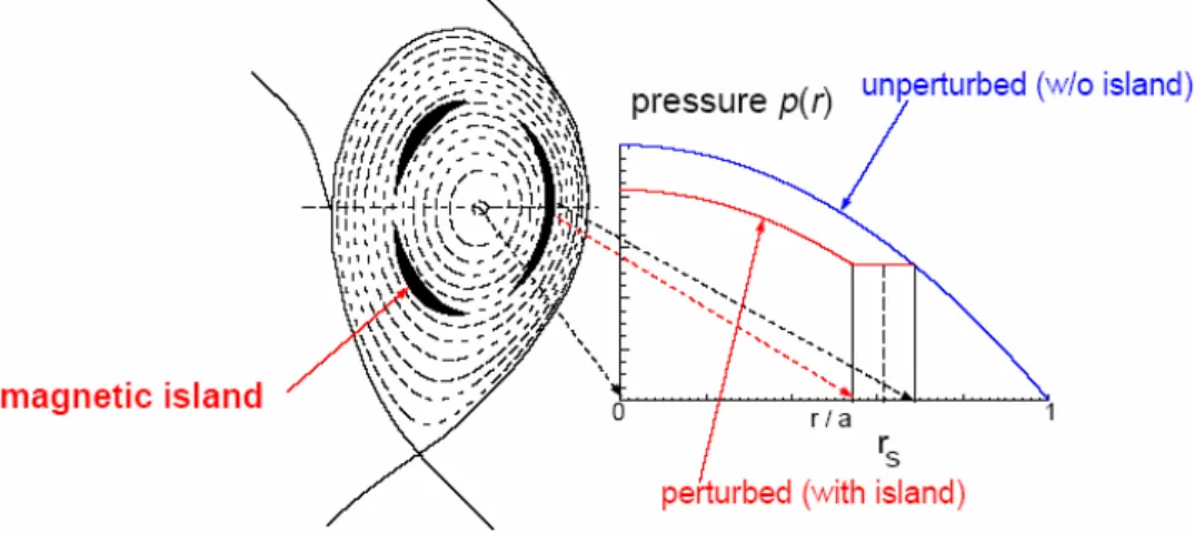
The effectiveness of the confinement is determined by the effective transport of heat and particles across the field lines. 7] proposed a model to describe the release of the crash, according to which the internal kink state will be driven unstable when the displacement of the magnetic field at theq = 1surfaces1 exceeds a certain critical value.

State of the art

• Actuator
• Model and experiments for sawtooth instability with fast particles
• Period locking
• Adaptive control and hysteresis
• Velocity distribution of the fast ions
• Physics oriented modelling
• Control oriented modelling

Instead of using a constant power wave deposition location, this controller manipulates the sawtooth period by modulating the power of the injected waves from the ECCD source. In another approach, the ECCD deposition location and the injected beam power were used as actuators [30].

Final goal and structure of this thesis

• Magnetic field diffusion
• Crash triggering
• Kadomtsev full reconnection model
• Witvoet Model input and output
• Implementation

The model uses only the magnetic diffusion equation to derive the evolution of the magnetic field. It is clear that this discontinuity quickly disappears due to the diffusion of the magnetic field. The shape of the magnetic field after the crash is determined from the shape before, using Kadomtsev's full reconnection model.

Lennholm model

This means that the output is only updated after each crash and remains stationary for the rest of the cycle. Consequently, there will be a delay between the code output and the corresponding input used, as it is necessary to wait until a new crash is triggered to determine the sawtooth period. The radial profile of the poloidal field is discretized into 200 points, using a denser distribution near the current mixing radius, which better describes the large diffusion taking place there.

Extended Witvoet model

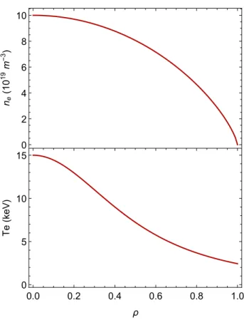
• Plasma quantities
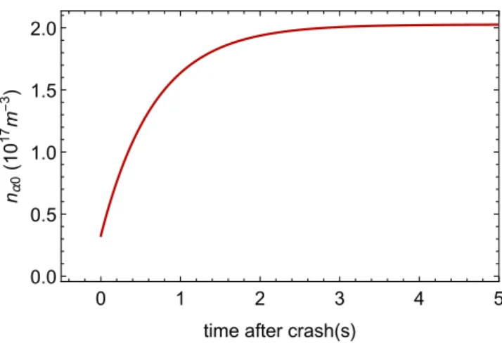
• Fast particles
• Triggering criteria
• ECCD
• ICRH
• Benchmarking

The total potential energy of the mode is given by the sum of five different components:. Therefore, it can be assumed that the location of wave deposition immediately follows the required value. First, Section 3.3.1 discusses the response of the extended Witvoet model with respect to this actuator only.

Analysis of the extended Witvoet model with ECCD

Response of the extended Witvoet model to ρ ECCD

If we want to keep this tokamak working efficiently, without tearing modes that degrade confinement, these long sawtooth collisions must be avoided, so some kind of actuation must be done to compensate for the stabilizing effect of these particles. . Thus, the current investigation focuses primarily on the development of a mechanism (or mechanisms) that can reduce the sawtooth period to values ​​of the order mentioned above.

Different ECCD configurations

As a result, the effect on the magnetic displacement from one source will also cancel out the effect from the other between each actuator, and therefore no improvement can be achieved with this method. As a result, the effect on the magnetic displacement from one source will also cancel the effect from the other actuator between the deposition locations of each actuator, where the driven currents cancel each other out. In fact, what we observe from the results in Figure 3.2 is that the greater the distance separating the two deposition sites, the lower the minimum period we get.

Conclusion

Analysis of the extended Witvoet model with ICRH

Response of the system to ρ ICRH

The larger of the two, the Graves term is only significant when theq= 1 the surface is close to the location of ICRH deposition, and thus continues to increase until ρ1 reaches ρICRD and the collision is triggered. Consequently, as the lower graph of Figure 3.6 now shows, after 35 seconds theq = 1 the surface is moving away from ρICRH and the Graves term is continuously decreasing, as the upper graph in the same figure shows. In order for the crash to trigger, you have to wait until Bussac's timer increases to compensate for it, which takes 250 seconds.

Response of the extended Witvoet model to both actuators

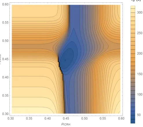
These controllers basically work by applying a change in actuator location that is proportional to the error, i.e. this method is based on the assumption that a positive variation of the actuator always leads to a change in the output in the same direction. Consequently, for ρICRH < 0.4∨ρICRH >0.7, the change in the sawtooth period due to the small variation of ρICRH is negligible and the gradient points vertically.

As found using only the ICRH actuator (Fig. 3.4), when ρICRH is far from the minimum, the Graves effect no longer has any effect on the collision initiation. In the graph below, the normalized radius of the area q= 1 is drawn next to the location of the ICRH and ECCD actuators. Consequently, after the same 53 s from the start of the second cycle, the critical shear is slightly above 1, so the collapse is not triggered at this time.

Chapter conclusion

Therefore, these methods require a detailed knowledge of the steady-state map and can only work in a limited area of ​​the map where the sign of the DC gain is constant. Second, it works by continuously estimating the DC gain, and thus does not require a detailed knowledge of the actuator storage location nor the steady-state map. In addition, the sawtooth period of most steady-state maps is very high, so it takes even longer to get some results, and this can make the controller extremely slow.

Extremum Seeking Controller

• Cost function
• Gradient estimator
• a) Moving average
• b) High pass filter
• c) Phase lag and gain compensation
• Optimizer
• Parameters tuning
• a) Perturbations
• b) Optimizer

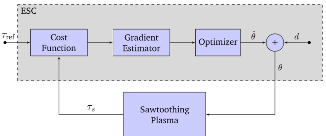
However, this would require knowledge of the steady state map in advance and would make the controller model dependent. To estimate the gradient of the cost function, a perturbation is added to the nominal operating pointθ, as illustrated in Figure 4.1:ˆ. The number of cycles required for the sawtooth period to converge was recorded and the simulation was repeated over the region of the steady state map where the gradient is larger.

Results

Reaching the minimum

To reach the minimum slack period, the cost function in ESC was removed. Since in practice it is very difficult to determine the precise actuator locations in real time, we had to assume that the controller can start at any location within a wide area of ​​the steady-state map. From these results, we can already conclude that the development of the controller towards the minimum is very dependent on the place where it starts.

For this purpose the steady-state sawtooth periodsτs(θ(k), t→ ∞) corresponding to the actuator location θ(k) at each time step is obtained from the steady-state map.

This shows that the relative difference is always less than 3%, i.e. the sawtooth period always converges to its steady state value and thus we can assume that the input-output dynamics is practically instantaneous. However, in the case of this simulation, the controller needed 60 time steps to reach the 50s sawtooth period mark, which is 20 time steps faster than in the first simulation.

The gray color marks the starting conditions from which the controller did not reach the minimum. This is because below this value the controller assumes the two-phase motion observed in simulation 6, and therefore this range should be avoided.

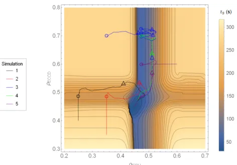
Avoiding local minima

The circles show the moments when local minima are detected, after which the amplitude of the perturbations increases over a period of approximately 50 time steps, culminating in the locations marked with triangles. It is important that the variation of the amplitude takes several disturbance periods, because it allows to cover a larger area of ​​the map than if a simple one. These results show that the global minimum of the sawtooth period can be reached regardless of the starting position of the actuators on the steady state map.

Testing the model dependency of the controller

This results in more irregular trajectories, as seen in simulations 1 and 2 in Figure 4.16 between the circle and the triangle. When this happens, if a local minimum is again detected, the process is repeated as it happened in simulation 3. However, it should be noted that the described process is very inefficient, since e.g. in simulation 3, 1000 steps were needed to reach the minimum.

Using this modified version of the model, we repeated the procedure explained in Chapter 3 to obtain a new steady state map. The evolution of the sawtooth period obtained in each simulation can be seen in Figure 4.20. Due to the similar shape of the input-output map, the controller behaved very similarly to the previous simulations.

Consequently, the optimizer goes directly to the minimum and not in stages as with the original model.

The plot of δWGraves0 as a function of the location of the q= 1 surface can be seen in Figure 4.24. The resulting steady state map is depicted in Figure 4.25 along with the controller trajectories in each simulation, starting from the same locations as in the previous cases. Again in 4 of the 6 cases the controller was able to reach the minimum in less than the 500 simulated steps.

Cost function

To prevent this, the controller would have to be tuned to the gradient it encounters. Apart from this aspect, the controller in the three examples presented here proved to be model independent, as it was able to reach the desired operating point (the one with the minimum sawtooth period) regardless of the changes made to the model. The case could be even worse if the previously requested period would lead the controller to one of the local minimums.

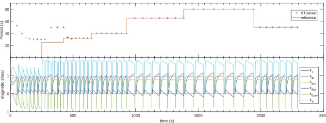
Period locking

For this reason, it is essential that both actuators are located in a region of the steady-state map where the sawtooth period is smaller than the reference period, preferably in the global minimum. The first step was to plot the steady-state map of the sawtooth period in response to the ECCD deposition location, using a fixed total driven current of 400 kA. In the second half of the thesis, the extended Witvoet model was used to develop a model-based controller for the sawtooth instability period.

Future work

Feedback control of the sawtooth period by real-time control of the ion cyclotron resonance frequency. Numerical demonstration of injection locking of the sawtooth period by means of modulated EC current drive. Real-time control of the sawtooth instability in fusion plasmas with large fast ion populations.

Evolution of the magnetic shear at the q = 1 surface and critical shear components for

Steady state map in a small region around the global minimum. The minimum sawtooth

Evolution of the quantities responsible for the triggering of the crash for ρ ICRH = 0.43 and

Overlap of two cycles shown in figure 3.8. The dashed curves represent the second, longer

Schematic representation of a typical ESC

Magnitude frequency response of a moving average filter with a time window of 10 crashes

Gradient of the cost function with respect to the first manipulated variable, ξ 1 , for the two

Schematic representation of the gradient estimator implemented

Schematic representation of the chosen optimizer

Schematic representation of the complete controller developed

Number of sawtooth cycles needed for the period to converge to the steady state value

Simulation results with different initial locations of the actuators. The lines represent

Difference between the steady state sawtooth period at the actuators location and the

Results from simulation 2 beginning with ρ ICRH = 0.43 and ρ ECCD = 0.55

Results from simulation 3 where the controller passes through the bifurcations

Results from simulation 6

Detailed results from simulation 4

Evolution of the nominal location of the controller in each simulation using the proposed

Comparison between fast particle density profile explained in chapter 2 with the new one

Sawtooth period obtained in each simulation, taking into account diffusion of fast particles. 59

Evolution of the nominal location of the controller in each simulation along with the steady

Evolution of the sawtooth period observed in each simulation using the new expression for