Deep Learning Techniques for Cell Stage Classification

The various phases and mechanisms that occur sequentially during the life of a cell form the cell cycle, and the correct progression along this cycle is essential for the maintenance of life. For a typical eukaryotic cell, this cycle can be divided into 2 main phases: interphase, in which the cell grows, and mitosis, in which the cell separates into two daughter cells.

List of Tables

Glossary

Introduction

Motivation

Objectives

Thesis Outline

Theoretical Background

Biological Background

• The Cell
• The Cell Cycle
• Cell Imaging
• Current cell staging techniques

On the inside of this membrane, the cytoplasm, a water-based fluid environment, makes up the interior of the cell. In contrast, if the DNA is in contact with the cytoplasm without any barrier, then the cell is prokaryotic. Along with G0, this phase of the cell cycle is the only one in which cells respond to extracellular stimuli.

If the cell enters a new round is made, the cell does not respond to external signals until the end of the cellular life cycle.[15]. The first phase participates early in the cell cycle and “licenses” the “origin points” by loading a pre-replicative complex onto the DNA. The M phase is the final stage of the cell cycle, after which two daughter cells will be generated from one parent cell.

During this phase, the cell's nuclear membrane collapses into various small vesicles that allow the mitotic spindle access to the chromosomes.

Machine Learning

• Deep Learning

These classification problems can be divided into two, supervised and unsupervised problems, depending on the shape of the training set [28]. It lacks a corresponding objective value that, in classification problems, corresponds to the target input class. Rather, they draw insights from our knowledge of the brain to arrive at models capable of statistical generalization.

As expression 2.5 clearly shows, the right choice of learning rate and momentum plays a crucial role in both the speed and success of training.[37] Convolutional networks use each kernel member at each input position, as shown in 2.10. A CNN can have one or several convolutional layers, the structure of which is represented in 2.12, depending on the complexity of the model.

This convolutional stage of the model is connected to an artificial neural network and the whole model is trained using the back-propagation method, similar to the explanation in the previous section.

Biological Material and Data

• Cell culture and imaging
• Image Pipeline

The images obtained from the fluorescence imaging were then processed to produce the data used as a starting point for this thesis. The image preprocessing pipeline described in figure 3.1 was used to process each FM image produced. Assuming that observations are independent and the noise obeys a Poisson distribution, the data can be described as:[45].

With the segmentation process, the cell culture images were divided into multiple images, each containing a cell nucleus. For these data, the segmentation strategy was used in the attenuated and contrast/intensity DAPI plane (blue channel) of the FM images and consisted in the application of Otsu thresholds and morphological operators to each image [43]. After all this processing was applied to each image, the obtained data were saved in a matlab file containing a pixel map for each nucleus and the corresponding binary classification from the FUCI method described in 2.1.4.

The information stored in these Matlab files formed the initial dataset for this thesis, consisting of 5873 grayscale images (since only the blue channel information was used) of the various nuclei contained in the initial images.

Methods

• Machine Learning

As such, training a network with elements can be viewed as training a set of 2-thinned networks with weight division. Thus, it is efficient to combine 2n networks into a larger single neural network that can be used at test time. There is no exact way to determine the value for each of the parameters, requiring an empirical process to determine the best solution for each problem.

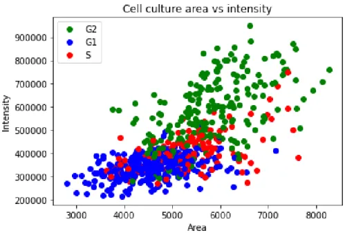
While not the only solution to overfitting deep neural networks, data augmentation addresses the problem at its root, the training dataset, by assuming that more information can be extracted from the original data by augmentation. One simple example of these techniques is isolating only the RGB channels or changing the intensity value of the image that describes the color histogram. Since the two most important features for describing cell cycle progression are surface area and intensity, careful selection of the techniques used is necessary to ensure that these features are not disturbed and adversely affect the outcome.

As such, from the methods described, only rotation, flipping and translations did not affect the area and intensity of the images used.

Validation

• MNIST dataset
• VGG Network

In addition to using the MNIST dataset for validation, a pre-trained VGG network was used as a benchmark for the convolutional neural network. The VGG network has an architecture with very small (3x3) convolutional filters followed by sixteen to nineteen weight layers and was proposed for the ImageNet challenge [56]. This challenge uses an example of the ImageNet dataset of about 1000 categories with 1000 images per category.

It represents an improvement over prior art (namely the AlexNet [57] network) and has become one of the benchmark networks for this challenge. Although the ImageNet challenge has a larger data set and is not exactly comparable to the data available for this project due to the difference in input format and number of channels used, the availability of various configurations of pre-trained VGG16- networks and the widely available biography about this network led to its selection as a benchmark.

Results

Artificial Neural Network

Although the validation set is above convergence accuracy, it corresponds to only 10% of the original dataset of ≈ 6000 points, which corresponds to a small amount. However, the accuracy of this method remains above 70% in every test set of the original data, which are promising results.

Convolutional Neural Network

As shown in Figure 4.3(a), the loss starts to decrease, but from about epoch 75 onwards it is clear that training is causing some overfitting. This can also be seen in Figure 4.3(b), where the validation accuracy starts to decrease while the training accuracy evolves. a) Evolution of losses per epoch (b) Evolution of accuracy per epoch. To simulate an early shutdown, the best performing network weights were saved and used to further fine-tune the network's training parameters to increase accuracy.

In particular, the learning rate was reduced to facilitate the convergence of the validation metrics with the training metrics. As shown in Figure 4.4, lowering the learning rate helped improve CNN accuracy and reduce its loss while preventing overfitting. Again, the weights of the best performing CNN were used to assess the network performance based on the same metrics as the ANN.

As stated in Section 3.3.2, the VGG network was used as a benchmark for CNN performance and trained on the same dataset with the same data augmentation conditions of the designed CNN.

Conclusions

Achievements

The ANN method relied on the manual extraction of intrinsic nuclear properties, area and intensity, which should adequately translate the cellular phase of an individual nucleus. Pooling fluorescence images from different cultures that were obtained at different times from cultures that might respond differently to the staining procedure was essential to unify the data set. In addition to the ANN method, two CNNs were also used in the thesis in connection with data augmentation techniques.

The first network was a self-designed simple CNN with only two convolutional layers that produced an accuracy of ≈87%, while the second network used was based on the architecture of a VGG network that achieved an accuracy of ≈83% delivered. Although the results achieved are still lower than those obtained with clustering algorithms, the increase in accuracy compared to the ANN still shows that using a CNN to address image-based cell classification is a promising solution. In particular, the further fine-tuning of the VGG network used can lead to accuracy results comparable to those achieved with clustering methods, as limited fine-tuning has been performed in this network due to its heavy computational requirements to train the development of it during this work.

Although below the results obtained with clustering methods, the results obtained with the proposed methods were very satisfactory and represent a promising solution to the problem of image-based cell classification for a single nucleus.

Future Work

Using this method, an accuracy of ≈ 76% was achieved in classifying cells in G1 or S/G2/M phase. The result, which is lower than the accuracy obtained with the clustering methods, still shows a clear correlation between the selected features and the cell phase. One possible explanation for this difference in accuracy is potentially the data normalization technique used.

However, due to this normalization, it is possible that some data points lost correlation between their features and the label. Both networks did not rely on manual feature extraction, but instead on automatic identification of features that translated cell phase.

Bibliography

Cell cycle control in mammalian cells: role of cyclins, cyclin-dependent kinases (cdks), growth suppressor genes and cyclin-dependent kinase inhibitors (ckis). Investigation of tadf properties of new donor-acceptor type pyrazine derivatives.Journal of the Chilean Chemical Society. The power and limits of deep learning: in his iri medal speech, Yann Lecun maps the development of machine learning techniques and suggests what the future may bring.

Prediction of wind pressure coefficients on building surfaces using artificial neural networks. Energy and buildings. Denoising total convex variation of poisson fluorescence confocal images with anisotropic filtering. IEEE Transactions on Image Processing. mnist database of handwritten digit images for machine learning search [best of the web].