Defesa de dissertação de mestrado: Victor Preuss

A software package for the steady-state simulation of autonomous circuits using the Harmonic Balance Method / Victor Hugo Bueno Preuss ; orientador, Fernando Rangel de Sousa, 2021. A software package for the steady-state simulation of autonomous circuits using the harmonic balance method.

SCOPE OF THE PROJECT

Main Goal

Envelope methods can be used for this kind of time-varying analysis using HB (NGOYA; LARCHEVEQUE, 1996). Concepts of model order reduction techniques are employed for circuit simulation to reduce the computational complexity of HB, as in Gad et al. 2000), and can be applied to problems of large size, where the Jacobian matrix may not fit the system memory, or the performance of its factorization becomes prohibitively slow.

Specific Goals

Dissertation Organization

There are different types of analysis that can be performed across a circuit and different types of input excitation are applied. Finally, section 2.5 comments on the Periodic Steady-State (PSS) analysis and the two main algorithms associated with it.

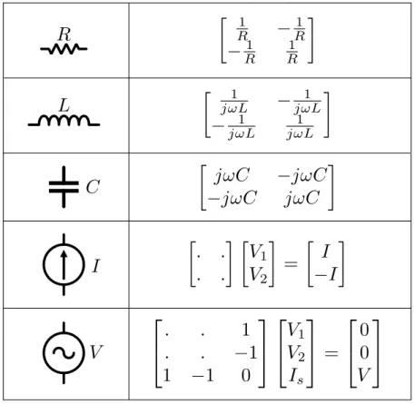
MODIFIED NODAL ANALYSIS

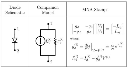
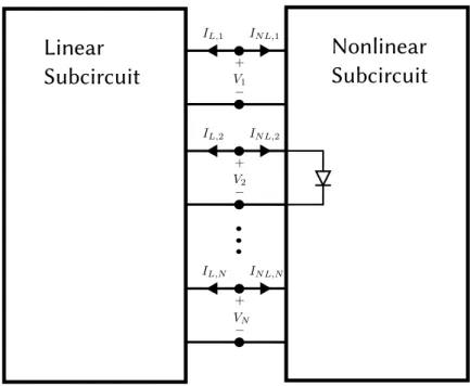
Except for the ground node, which adds no information to the system, and using the stamps from Figure 1, the matrix system in Equation 3 can be assembled automatically by a computer, simply by placing the stamps on the correct nodes. Although the presented example is for a simple linear network, the stamping method for the MNA system can be extended to support dynamic elements of time-varying nature and also non-linear entities by using a linearized version of the system with an iterative solution.

DC ANALYSIS

Newton-Raphson Iteration

Assuming a candidate solution V(i) exists for the system in Equation 6, the Newton-Raphson iteration formula can be written as,. A more physical interpretation is that Newton-Raphson performs a linearization of the circuit equations over V(i) and improves the solution approximation by going in the direction of minimizing F(V).

Limiting the Range of Device Models

This approach effectively limits the variation of the exponential function to ±10φT per iteration, greatly improving the stability of the exponential.

Continuation Methods

Source Stepping
g min Stepping

AC ANALYSIS

This is not the case with an HB run, so models must be able to handle very large variations in voltage and current (MAAS, 2003). AC analyzes are usually performed using frequency sweeps, therefore the complex part of the stamps that depends on jω has to be recalculated at each frequency value.

TRANSIENT ANALYSIS

Therefore, all that is required to perform an AC analysis is to create the MNA matrices. Since the problem of finding the transient solution Vk+1 is implicit (Ik+1 is required to predict Vk+1), the Newton-Raphson iteration is required to solve the MNA system, regardless of the presence of nonlinearities.

PERIODIC STEADY-STATE ANALYSIS

This was one of the main motivations cited by Nakhla and Vlach (1976), who introduced the Piecewise Harmonic Balance algorithm. Linear elements can be treated directly in the frequency domain using phasor analysis, while non-linear devices use their time domain models using the Discrete Fourier Transform (DFT).

AN INTRODUCTORY EXAMPLE TO HARMONIC BALANCE

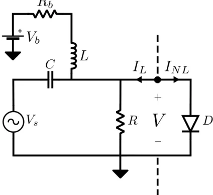
IL(kω) +IN L(kω) = 0 for k= 0.1, .., K (19) Assuming that V(kω) is the node voltage phasor at frequency kω, the current flowing in the linear circuit for every harmonic can be calculated,. For a nonlinear current flowing through a diode, the amplitude of the current phasor for each harmonic can be found using the results of Clarke and Hess (1971).

THE HARMONIC BALANCE ALGORITHM

Notation

The Discrete Fourier Transform

Single-Tone Nodal Analysis

Including Voltage Sources

The charge derivative term is required to calculate the current contribution of the nonlinear capacitances. The next term to examine is the convolution integral responsible for the current contribution of the linear elements.

Numerical Solution of the HB Equations

The Newton-Raphson Approach
Termination Criteria

If we also expand the complex phasors in G and C into their R2 representations, equation 49 can be rewritten as,. I(V) =Γ×i(v) = Γ×i(Γ−1V) (63) Using the chain rule of differentiation for Equation 63, G can be expressed in terms of the time domain current sink. V(i+1) =V(i)−J(V(i))−1F(V(i)) (70) Therefore, starting with a guess for V(0), the Jacobian J(0) is calculated using equations 54 and NR iteration can be used to continuously improve the stress guess until a solution is reached.

Convergence of the harmonic balance analysis is achieved when the error obtained in F(V) can be neglected.

HB for Multi-Tone Excitation

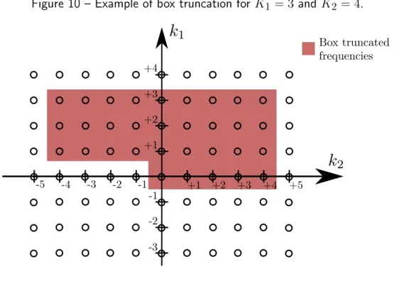
Box Truncation Scheme
Artificial Frequency Mapping

Therefore, the main insight of the AFM technique is that, if the Fourier coefficients do not depend on the actual frequency, one can choose a convenient frequency value, λ0, to perform the DFT, over which the sequence of frequencies ΛK is actually dense and periodic . Nevertheless, at the end of a simulation, the trigonometric form of the obtained Fourier coefficients can be used to calculate the correct time-domain response. The rest of the HB algorithm, which is performed in the frequency domain, is done entirely over the set ΛK, including constructing the admission matrix Y.

This case is handled by always taking the absolute value of the frequency to perform the calculations, and after the DFT is applied, the complex conjugate Fourier coefficient of these terms is used.

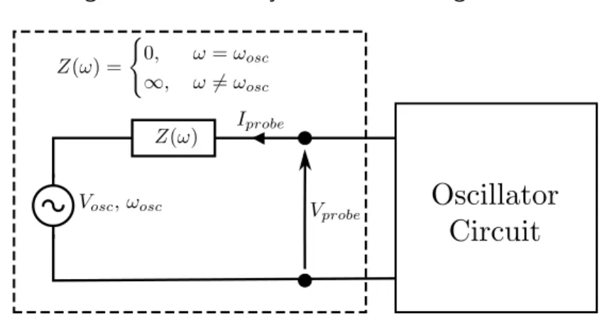
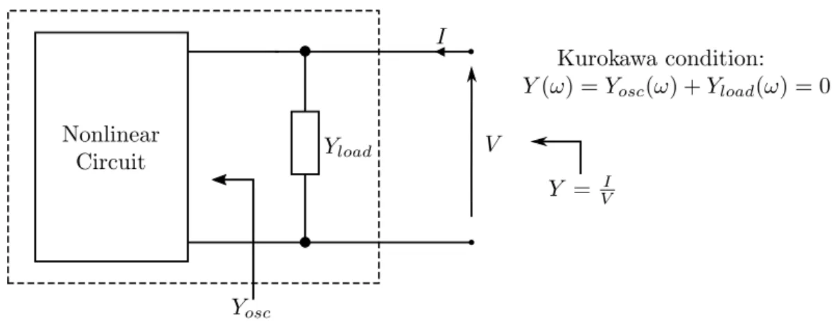
Including Autonomous Circuit Support

Vosc(ωosc) =|Vosc|ejφosc (89) Since there is a generator with a defined frequency ωosc, the HB formulation of the oscillator circuit with the connected probe can be written in the short format. The core idea of the method is based on the fact that the existence of the probe must not disturb the stationary regime of the oscillator. This can be ensured by making the probe's fundamental frequency allowance equal to zero, since the probe already does not disturb the other harmonics.

Vprobe(ωosc) = 0 (91), where the value of Iprobe is a product of the HB simulation, while the auxiliary generator.

Improvements in Convergence

Initial Guess
Source Stepping

Because of his heavy involvement in areas like machine learning and data science, there are plenty of resources available for Python developers/learners, making it more accessible for other people to contribute to this project over time. Additionally, Python allows writing highly readable and clean code that invites new users to understand the inner workings of the circuit simulation engine. Finally, the existence of three other tools: scikit-rf (ARSENOVIC, 2009), SignalIntegrity (PUPALAIKIS, 2018) and openEMS (LIEBIG et al., 2013) was also important for the use of Python in this project.

Due to the research nature of this project, performance was not a top requirement for the current implementation.

OVERVIEW OF IMPLEMENTED ALGORITHMS AND DEVICES

DC Analysis
AC Analysis
Transient Analysis
Harmonic Balance Analysis

The creation of the DFT/IDFT and Ω matrices is straightforward after the frequency basis is known. The frequency of the AC currents must be checked against the fundamentals set on the simulation, as there can be no excitation frequency outside the frequency fundamental. Finally, for the setup phase, an initial condition given by the user or based on the DC solution of the circuit is used to initialize the voltage array.

The purpose of this objective function is to take a guess for the frequency and magnitude of the oscillation at the probe node, apply it to a harmonic balance simulation, and return the total probe admittance.

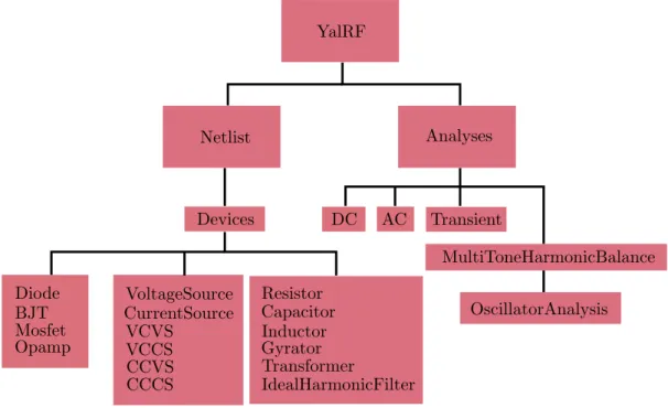
YALRF CODE ORGANIZATION

The Analyzes library on the chart contains the implemented algorithms for each analysis currently supported. The creation of an abstract class for the analyzes can be considered later to standardize the way the user interacts with the algorithms. The first section presents the analysis of a simple differential amplifier using DC, AC and HB simulation.

The next section presents the design of multiple oscillator circuits with their steady-state response obtained using YalRF's implementation of the Auxiliary Generator technique.

CASE STUDY: DIFFERENTIAL AMPLIFIER

DC Operating Point

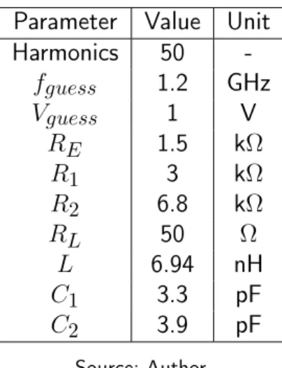
This chapter presents simulation results of some topologies using YalRF and some comparisons are made with Keysight's ADS and QucsStudio. Finally, a diode demodulator example presents the two tone characteristic of the HB simulation, using the artificial frequency mapping method for the Fourier transformation of quasiperiodic signals. The results agree very well, which works as a good validation of the DC part of the BJT model.

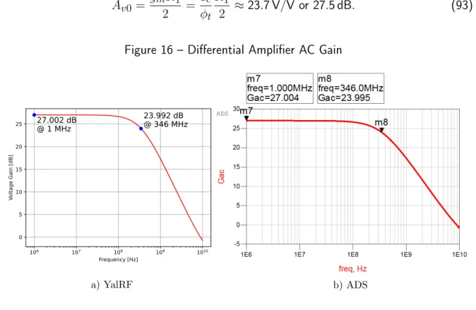
AC Gain and Gain Compression

To obtain this simulation result, an input voltage sweep is performed using harmonic balance simulation, and the large-signal gain of the amplifier is calculated by taking only the first harmonic magnitude of the input and output. As the input signal begins to rise, nonlinearities begin to occur and effectively distort the output signal of the amplifier. If the base-emitter voltage swing becomes large enough, the small-signal assumption used in the gain calculation is no longer true, as the exponential characteristic of the BJT begins to generate multiple harmonics.

For the parameter sweep, the solution from the previous iteration was reused as the initial condition for the next one.

CASE STUDY: OSCILLATOR ANALYSIS USING HARMONIC BALANCE 67

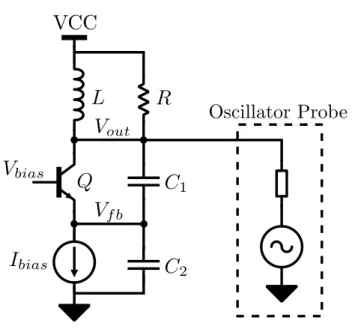
Common-Base Colpitts Oscillator

Small-Signal Analysis
Large-Signal Analysis
Simulation Results
Automatic Design Optimization
Oscillator Results using a BJT Model with Nonlinear Parasitics

The negative resistance of the Colpitts oscillator of Figure 24 is generated by the transistor Q and the feedback capacitive divider. The non-linear mechanism which limits the oscillation amplitude of the Colpitts from Figure 24 is the reduction of the transistor transconductance for large signals. As seen in Figure 32, the Colpitt's oscillator efficiency has an optimum value of about 0.1.

The results obtained for the optimization of Colpitt's oscillator efficiency are presented in Table 7.

Common-Collector Colpitts Oscillator

The output taken at the 50 ohm load, shown in Figures 40 and 41, has been deliberately kept very distorted, to show that the algorithm converges for high non-linearity distortions. The fact that the time-domain signals are quite similar confirms that the phase of each harmonic component is correct. Subtle differences on the time-domain waveform can be attributed to two separate factors: first, the oversampling value used to reconstruct the time-domain waveforms is probably different.

Second, ADS uses the FFT algorithm to calculate the time-frequency conversions instead of the DFT matrix used in YalRF.

Peltz Oscillator

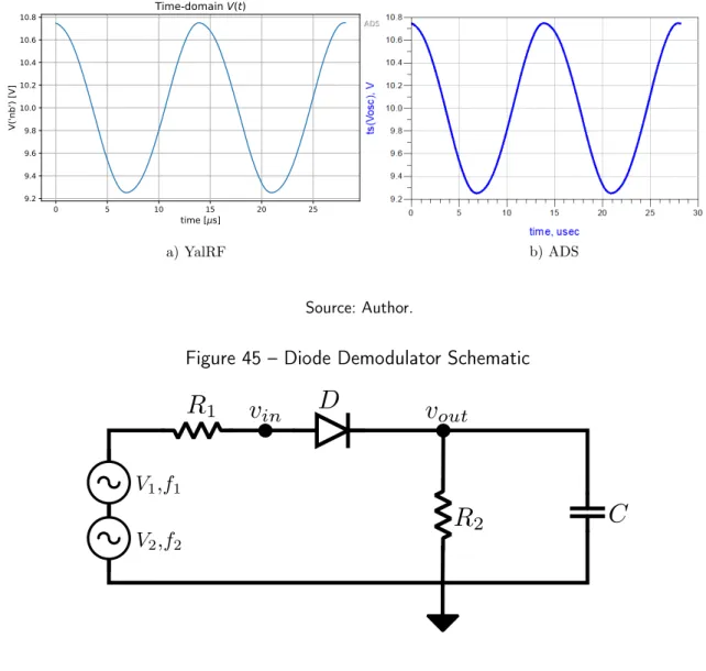
CASE STUDY: DIODE DEMODULATOR

The two-color feature of the HB simulation requires more in-depth testing, but the results obtained so far indicate a good agreement with ADS and QucsStudio implementations. A more in-depth review of the HB technique was performed and a two-tone version of the algorithm was implemented. The fast convergence of the HB for different levels of excitation showed a good stability of the implementation.

The obtained results proved the application of the frequency map used for quasi-periodic signals.

FUTURE WORK

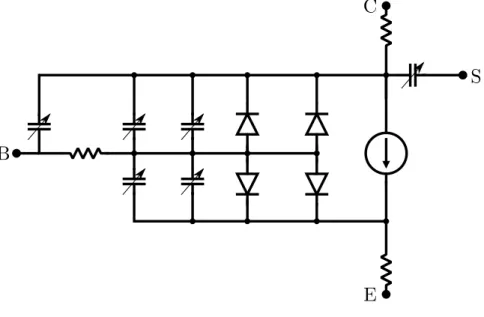
In this context, this thesis worked as a very broad introduction to the field of circuit simulation, and greatly contributed to the author's formation with a view to future state-of-the-art work. This circuit is an approximate model of the input of a common-emitter amplifier stage using a BJT, where the diode represents the base-emitter junction. The frequency-domain derivative of the current phasors with respect to the stress phasors were calculated using a Secant approximation, which can be written as, .

This section presents the Python code used for some of the test benches presented in Chapter 5.