Design and Simulation of an ABS Control Scheme for a Formula Student Prototype

O modelo é integrado à dinâmica da linha de freio e a um modelo de atrito dos pneus baseado em dados experimentais confiáveis. Palavras-chave: sistema de frenagem ABS, Fórmula Student, controlador fuzzy, controlador PID, estimativa de patinagem de rodas, modelo de veículo, modelo de pneu.

List of Symbols

Acronyms

Introduction

• Brief history of ABS
• Motivation (Formula Student)
• Objective
• Work contributions
• Outline

An in-house developed vehicle model with 14 degrees of freedom (DOFs) was built for ABS design and subsequent simulation. Brake line dynamics relevant to ABS design were modeled and integrated into the complete vehicle model.

Vehicle Dynamics

• Global Overview
• Horizontal Dynamics
• Vertical Dynamics
• Lagrange Method
• Vehicle Loads
• Inverse Kinematics
• Tire Vertical Load
• Wheel Dynamics
• Free-body diagram
• Brakeline Dynamics
• Steady-state equations
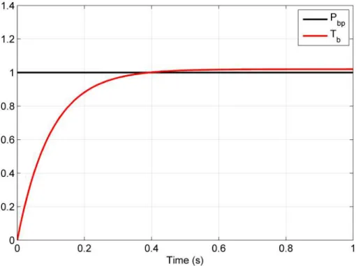
• Transient behaviour
• Hydraulic Modulator

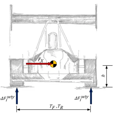
Tire model is an empirical model of the complex frictional dynamics between the tire and the pavement. This enables a real-time calculation of the tire load when the vehicle is subjected to dynamics (load transfer and aerodynamics). As the car accelerates, inertial forces are generated on the CG by the sprung and unsprung masses.

Using the longitudinal load transfer free-body diagram shown in Fig. As described at the beginning of this chapter, Wheel Dynamics employs the sum of forces and moments acting on the wheel to calculate the angular velocity of the wheel ωW. With knowledge of the coefficient of friction between the brake pads and the rotor, µpads, the braking torque is finally calculated.

Tire Model

Types of models

• Pacejka Model
• Burkhardt Model
• Neural Network Model

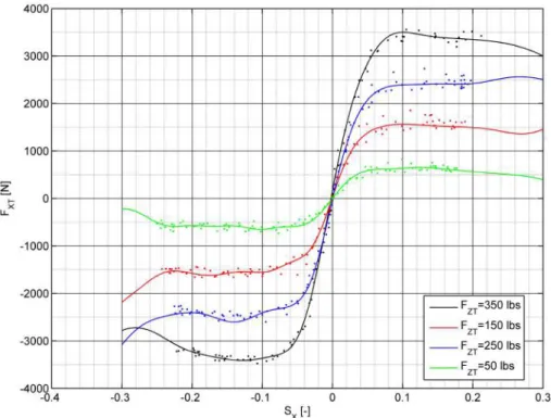
Pacejka1 tire model [13] is the most widely used tire model to calculate steady-state tire force and moment characteristics for use in vehicle dynamics. When multiple inputs are required for the tire model (e.g. varying vertical tire load and road friction coefficient are important for this application), the aforementioned parameters themselves are given by parametric functions (of parameterspi,qi,ri orsi) whose inputs are the supplementary input variables FZT,γand p . In this thesis, only the first case for the development of the tire model is considered.

Although this model takes into account the influence of the vehicle speedv on the friction curve, there is no dependence on the tire vertical loadFZT or inclination angleγ. To take advantage of the effectiveness of ANN for non-linear curve fitting, a band model using this type of soft computing algorithm was developed. A model of this kind is not only relatively quick to develop, it also allows the use of any mapping combination of variables as in the Pacejka tire model.

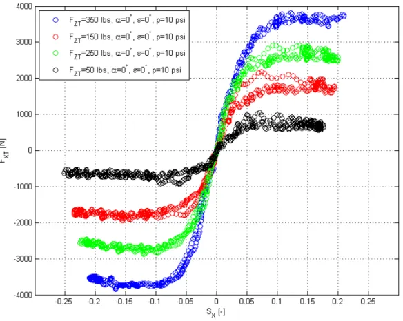
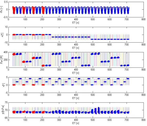
Experimental Data

As described, there is an SXsweep for each of the possible combinations of the other 4 variables, α, FZT, γ, and p, as a sequence of cycles.

Data Fitting

• Methodology for Pacejka and Burckhardt models
• Results

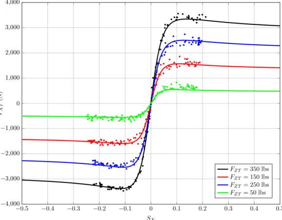
The best fit in terms of least squares is the parameter column vectorsp=pit, which minimizes the sum of squares of the residuals, i.e. the difference between the experimental value and the fitted value provided by the model. As in the Pacejka model, the parametric expression defining the Burkhardt model (Eq. 3.4) is specific to tire assembly, i.e. qualitatively correct. However, the poor fit to the limits of the experimental data suggests that extrapolation is not recommended in this case.

Nevertheless, using the same values ​​for the coefficients [A, B, C, D], Burkhardt model is useful to reproduce the influence of the velocity on the tire force. After several iterations of different trained ANN, the network with the best fit was selected. Considering the results obtained with the three tire models, a decision was made on the Pacejka model to be connected to the complete vehicle model for the design and simulation of the ABS controller.

ABS Overview

• Objectives of ABS
• ABS Components
• Wheel Slip Control
• Longitudinal Slip Ratio
• Control Problem Definition
• Main difficulties
• Control Methods
• Threshold Control
• PID Control
• Sliding-mode Control
• Intelligent Control

The complete set of closed-loop variables for wheel slip control is listed in Table 4.1. Another significant aspect is the fact that the system is unstable for wheel slip values ​​beyond the peak friction force seen in Fig. From the detailed issues discussed above, wheel slip control is indeed a very complex and challenging problem.

A gray sliding-mode controller is designed by Kayacanet al[23] to maintain wheel slip at the desired value. The proposed structure includes a gray prediction to anticipate the upcoming speed-dependent values ​​of wheel slip and reference wheel slip. An optimized fuzzy controller is proposed by Mirzaeiet al [3] to maintain wheel slip at a desired level.

Proposed Approach

Problem data and requirements

• FS Rules
• Competition characteristics
• FST 05e

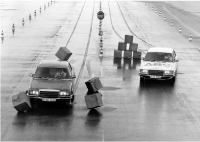
The braking system must be capable of locking all four wheels during the Braking Test, i.e. it must be able to turn off the ABS. As most of the dynamic events are fixed and the circuit layout is, at least in part, known from previous races, it is possible to accurately reproduce competition conditions, including the load cases the car will be subjected to and the dynamics relevant. behavior. In addition to the known parameters of the target vehicle, listed in table 7.1, the specifications on the brakes.

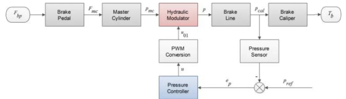
The prototype has two independent hydraulic braking circuits for the front and rear wheels respectively. The brake pedal operates on the master cylinders, one for each circuit, and hydraulic pressure is transmitted via rigid brake lines to a floating caliper on each wheel.

Proposed Control Structure

• Inner Loop - Brake Pressure Controller
• Outter Loop - Wheel Slip Controller

The brake system represents only the brake line dynamics (Section 2.5), while the vehicle model includes the remaining horizontal, vertical and wheel dynamics and the tire model described in Section 3. No overshoot, which could lead to excessive braking and consequently the wheel being in an unstable area of ​​the tire friction curve (Section 4.3.3). The wheel slip controller in the current cascade structure works by calculating the reference pressure based on the wheel slip erroreSX to a given reference SXref.

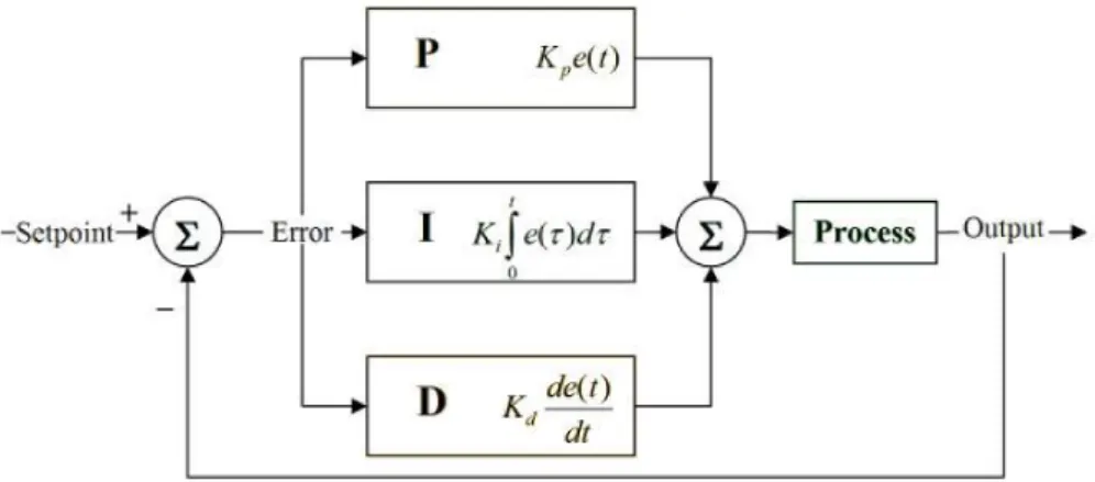
A PID-type fuzzy controller with a Takagi-Sugeno-Kang (TSK) fuzzy system is proposed here to maintain wheel slip at a desired value (Fig. 5.5). 5.5, the input variables of the fuzzy controller (also linguistic variables) are the wheel slip error erroreSX =SXref−SX and its variation∆eSX within a time stepT. In turn, the FIS output is multiplied by the gainK∆p before integration.

Design Approach

It is preferable to choose pressure variation rather than directly derive the reference pressure because the optimal value varies with vehicle speed. The PID type classification is related to the fact that, before entering into the FIS, both input variables are multiplied by the gainsKeandK∆e, which corresponds to the proportional and derivative gains of a PID controller.

ABS Design

• Brake Pressure Controller
• PID Overview
• PWM Conversion
• Open/closed loop step response
• PD Design
• Wheel Slip Controller
• FIS Overview
• FIS Design
• PID Gains Optimization
• Reference Wheel Slip
• Wheel Slip Estimator
• Complementary Filter
• ABS Triggers
• Minimum brake pressure
• Wheel slip and wheel slip rate trigger
• Low velocity trigger

Critical Gain (Closed Loop) — The integral action cannot be separated from the system, so the system never becomes unstable. Recalling the closed-loop step response characteristics in Section 6.1.3 (no steady-state error), the integrated gain is not included. Therefore, the procedures involved in the calculation of the output signals are also different between Mamdani and TSK fuzzy systems.

A1 Negative eSX < SX is below the reference slip, within the stable area of ​​the tire friction curve (brake pressure too low). A3 Positive eSX >0 1 0.425 SX above the reference slip, within the unstable region of the tire friction curve (brake pressure too high). An alternative method is to use direct integration of the longitudinal acceleration measurement provided by the mounted accelerometer as shown in Fig.

Simulation Results and Analysis

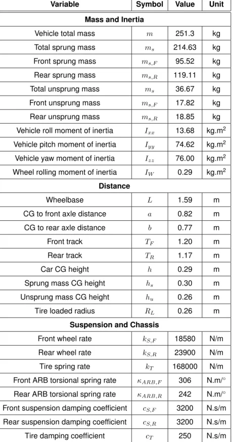
Simulation Parameters

• FST 05e Parameters

Straight Line Hard Braking

• Constant µ
• Varying µ
• Without pressure controller

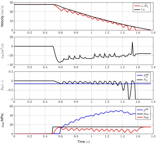
If the vehicle is equipped with ABS, the wheel speed is reduced so quickly, until the reference slip SXref =−0.16 is matched and efficiently tracked. The ramp rate is then slowed down to avoid overshoot when the wheel slip approaches the reference value. Since the pressure must be released to counteract this effect, the slip controller immediately reduces the reference pressure.

After a short underpressure, reference pressure stabilizes near 5 MPain for about 0.1 s and wheel slip is restored to the reference slip value. As wheel slip is now within the stable region, the reference pressure is increased more slowly and tracked without overshoot, with wheel slip settling in 0.2 s. Even if the wheel slip controller's gains are not optimized as they cannot handle the hydraulic deceleration dynamics, simulation results show continuous oscillation of the wheel slip around the reference value instead of settling.

Complete Lap

To simulate the ABS system without the inner loop, the reference pressure variance ∆prefb is fed directly into the hydraulic modulator as the command signal, as depicted in Fig. On the other hand, if equipped with an ABS, not only does the driver benefit from maximum braking power at every corner, even if he presses the brake pedal hard, but controllability is also guaranteed. In terms of GG diagrams, the shape is narrower and closer to a cross in the case without ABS (Fig.

With the ABS on, the driver can brake later, which is shown by the longer parts of the trajectory in red, and most often already in the corner. The lap time results for each simulation are listed in Table 7.5, with a significant difference of almost 4 s/lap. 2The Endurance event is the main FS event designed to evaluate the overall performance of the car and to test the durability and reliability of the car.

Summary and Conclusions

Future work and research

As mentioned in the thesis objectives in section 1.3, the physical implementation of the proposed controller was a concern. A balancing algorithm must then be implemented so that even the tire forces on the right and left sides of the car are always prioritized. As an electric vehicle, the FST 05e uses an electric motor to drive each of the rear wheels, which can cause significant inertial effects during braking that have not been investigated.

Oscillations around the reference wheel slip, mainly during the transient period, correspond to oscillations in the acceleration of the car's CG, which in turn are transmitted to the suspension due to weight transfer. A comparative study between the frequency of these oscillations and the natural frequency of the car's suspension can be carried out using the vibration model described in Section 2.3. Results can be evaluated either in terms of the driver comfort or ABS improvement with an active suspension system, as proposed in [30].

Bibliography

Sadeghi, “The design of a sliding mode controller for anti-lock braking system,” in The International Conference on Computer as a Tool (EUROCON), vol. Datta, “Sliding mode controller for wheel-slip control of anti-lock braking system,” in IEEE International Conference on Advanced Communication Control and Computing Technologies (ICACCCT), Aug 2012, pp. Yaghoobi, “A new approach in anti-lock braking system (ABS) based on adaptive neuro-fuzzy self-tuning PID controller,” in 2nd International Conference on Control, Instrumentation and Automation (ICCIA), Dec 2011, pp.

Gao, “An adaptive nonlinear filter approach to the vehicle speed estimation for ABS,” inProceedings of the 2000 IEEE International Conference on Control Applications, 2000, pp. Xu, “Vehicle speed estimation based on adaptive Kalman filter,” inInternational Conference on Computer, Mechatronics, Control and Electronic Engineering (CMCE), vol. Moaveni, “Vehicle Speed ​​Estimation Based on Data Fusion by Kalman Filtering for ABS,” in 20th Iranian Conference on Electrical Engineering (ICEE), May 2012, pp.

Appendix A

SAE Definitions

Axis Systems

• Earth-Fixed Axis System
• Vehicle Axis System
• Intermediate Axis System
• Tire Axis System

The intermediate axis system is used to facilitate angular turns using the Euler angles of the vehicle and the definition of angular orientation terms, the components of force and moment vectors, and the components of translational and angular motion vectors.

Angles

• Vehicle Orientation
• Tire Orientation

Yaw Angle (Heading Angle),ψ The angle from the XE axis to the X axis, around the ZE axis. Note: The pitch angle is not measured relative to the road surface, so a vehicle resting on a.