First, a temperature-controlled structure was constructed to improve direct MCE measurements by means of the adiabatic temperature change, Δ𝑇ad. Gadolinium measurements of the standard magnetocaloric material (Gd) and one of the most promising magnetic coolants, MnFe(P,As), are investigated.
RESUMO
ACKNOWLEDGEMENTS
I am grateful for the design and technical assistance of Marcelo Ribeiro, especially for the rotary valve and regenerator designs. I thank Pedro Magalhães for his kindness and cheerful support, especially in the uncertainty analysis.
LIST OF TABLES
LIST OF SYMBOLS AND ABBREVIATIONS
CONTENTS
INTRODUCTION
MOTIVATION AND OBJECTIVES
The design of such thermomagnetic systems depends on a large number of geometric, magnetic and hydraulic variables, for example those summarized in Table 1. As will be seen, a significant effort has been devoted to the design of optimized magnetic systems in this thesis. circuits and hydraulic power distribution systems.
THESIS OVERVIEW
Appendix B presents the characterization of the Gd spheres used in the UFSC magnetic refrigerator.

LITERATURE REVIEW
FUNDAMENTALS OF THE MAGNETOCALORIC EFFECT The magnetocaloric effect (MCE) is the thermal response of
- Thermodynamics of the magnetocaloric effect When the material is magnetized adiabatically, the ordering
- Experimental characterization of the MCE
2.3) can be integrated to find the entropy change if the specific heat capacity is known as a function of temperature and magnetic field. This approach requires magnetization data as a function of temperature and magnetic field which is easily obtained from commercial magnetometers, such as SQUID (Superconducting Quantum Interference Device) or VSM (Vibrating Sample Magnetometer).
MAGNETOCALORIC MATERIALS
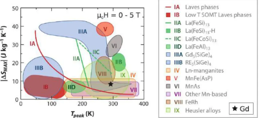
- Gadolinium (Gd)
- Promising magnetocaloric materials
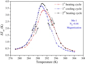
Second-order materials have a reversible MCE (Bahl & Nielsen, 2009), while some first-order materials can have an irreversible MCE due to hysteretic losses (Morrison et al., 2009). The maximum point of Δ𝑇ad is close to 𝑇C and increases with Δ𝐻 (Pecharsky et al., 2001).

Magnetocaloric Materials
NaZn 13 -type structure system
Intermetallic lanthanum-based compounds, such as La(Fe,Si)13, which crystallize in the NaZn13-type structure (1:13 phase) (Palstraet al., 1984), and the transition metal-based compounds MnFe(P, As ), which crystallize in the Fe2P type structure (Tegus et al., 2002), are among the most promising magnetic coolants for near-room temperature magnetic cooling. Other studies have investigated these magnetocaloric compounds and their application in magnetic refrigerators (Shenet al., 2009; Liu et al., 2012).
Fe 2 P-type structure system
Concerns about toxicity (arsenic) led to the complete replacement of this element with silicon (Si) and germanium (Ge), while still maintaining the same crystal structure and high MCE at room temperature (Teguset al., 2004; Dagulaet et al. ., 2005; CamThanhet et al., 2006; Lozano, 2009). Figure 7 shows the magnetization as a function of temperature for MnFeP0.45As0.55, which has a much more abrupt transition than the (smooth) second-order transition of Gd.
REGENERATORS
Thus, a fixed spatial fraction of the matrix is in the hot bladder, while another fraction is in the cold bladder. In this case, the fluid can be pumped continuously from one side of the matrix to the other, as shown in Fig.

ACTIVE MAGNETIC REGENERATOR (AMR)
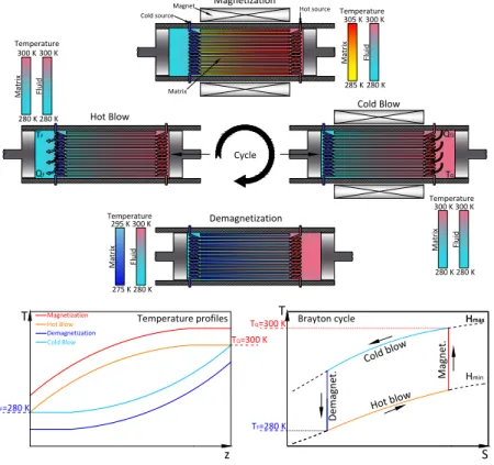
Each cross-sectional segment of the magnetocaloric matrix in an AMR undergoes a Brayton cycle over a small temperature difference corresponding to the Δ𝑇ad of the magnetocaloric material at the local temperature and magnetic field change. Adiabatic Magnetization: By adiabatically increasing the magnetic field applied to the regenerator, the total entropy of the magnetic solid matrix remains constant.
MAGNETIC REFRIGERATORS
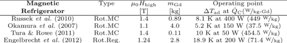
- State-of-the-art magnetic refrigerators
- Astronautics – USA system
- Japanese system
- Canadian system
- Danish system
Machine photo (left side) and AMR flow diagram (right side). Among the most modern magnetic refrigerators developed so far, special attention is paid to the Danish system, which was experimentally and numerically evaluated in the thesis.
AMR MODELING
The terms represent (from left to right) the fluid enthalpy change due to advection, interstitial heat transfer with the solid, energy storage, energy transfer due to axial dispersion associated with mixing of the fluid, and viscous dissipation due to frictional losses. The terms (from left to right) represent the interstitial heat transfer with the flowing fluid, nondispersive or static axial conduction (through matrix and fluid), magnetic work transfer, and energy storage. It is worth highlighting the importance of knowing the exact behavior of the properties of solid refrigerant samples used in experimental units for an accurate prediction and interpretation of thermal performance results.
MAGNETIC CIRCUITS FOR MAGNETIC REFRIGERATORS Magnetic field changes are the driving force in a magnetic
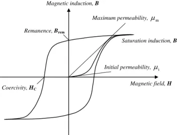
- Fundamentals of magnetism and magnetic materials Magnetism is the physical phenomena of substances in re-
- Demagnetization field
- Modeling a magnetic circuit
- Desired characteristics of a magnetic circuit for a magnetic refrigerator
- State-of-the-art magnetic circuits
Some of the magnetic circuits designed and built for this purpose are presented in Section 2.7.5. It is also very important for the magnetic circuit to have a large area with a low magnetic field, since the MCE of the magnetocaloric material is proportional to the magnetic field change. This section presents some modern magnetic circuits developed for magnetic cooling applications.
SUMMARY AND SPECIFIC OBJECTIVES
Investigate the influence of AMR parameters through analytical and numerical simulations to aid in the design of magnetic cooler components; Experimentally characterize the magnetic cooler under different operating conditions of temperature, frequency and flow. Develop a method to evaluate the thermodynamic efficiency of magnetic refrigeration devices and apply it to a state-of-the-art magnetic refrigerator.
DIRECT MEASUREMENT OF THE MAGNETOCALORIC EFFECT
- DIRECT MEASUREMENT OF THE MCE
- EXPERIMENTAL APPARATUS AND PROCEDURE
- EXPERIMENTAL WORK
- RESULTS .1 Gd samples
- Mn-based samples
- SUMMARY
The effect of the shape of the sample on the magnetic field is taken into account by the average demagnetization factor of the sample, 𝑁𝐷. The corresponding dimensions and demagnetization factors of the samples tested in this work are summarized in Table 6. 37 shows the change in adiabatic temperature of three Mn-based samples with different compositions and different Curie temperatures.

DESIGNING A NOVEL ROTARY MAGNETIC REFRIGERATOR
DESIGN CONCEPTS
The rotating magnetic circuit-stationary regenerator configuration was chosen for the present study due to the following characteristics: (i) higher operating frequencies with low magnetic strengths, (ii) higher magnetized volume, (iii) pumping fluid flow with less leakage, (iv) compactness, and (v) a magnetic circuit with more efficient use of magnets. The desired flow rate of the glycol solution is set by a gear pump controlled by a frequency inverter and a flow bypass. In this way the flow distribution system works continuously and the magnet is used most of the time.

INITIAL DESIGN CONSTRAINTS AND SPECIFICATIONS As suggested by Rowe & Barclay (2002), the design of a mag-
The design of the AMR mainly depends on the interaction between the magnetic circuit, the current distribution and the sizing of the regenerator. For example, the applied magnetic field is inversely proportional to the height of the magnetic gap, which is clearly a limitation on the regenerator height. The single pressure drop and pump power as a function of bed length for different particle diameters and 𝜑= 1.0 (𝜀=0.36) are shown in Fig.

DESIGNING THE MAGNETIC CIRCUIT
- Optimization of the rotor-stator magnetic circuit configuration
The properties of the soft magnetic material needed in the magnetic circuit simulations were identical to those of iron. The magnetic flux density and energy product of the basic rotor-stator configuration are shown in the figure. The 2D simulated average energy product of the permanent magnet in the basic magnetic circuit is 192.8 kJ/m3 (Figure 46-b).

BASIC PROPERTIES
- Characterization of the magnetic circuit
- DESIGNING THE FLOW DISTRIBUTION SYSTEM The flow distribution system is responsible for the alternat-
- Designing the rotary valve system
- Designing the flow distributors and the cold end The absence of a rotary valve at the cold end requires the use
- DESIGNING THE REGENERATOR
- Adapting a 1D numerical AMR model
- Final dimensions of the regenerator
- Assembling the regenerator
- ANCILLARY COMPONENTS
- Thermal components
- Driver system
- Instrumentation and control components
- Equipment information
- PRESSURE DROP ANALYSIS
The magnetic flux density ratio of the final magnetic circuit from the 2D simulations is shown in Fig. The magnetic flux density is calculated as: i) 2D area average, (ii) 3D volume average, and (iii) 3D magnetic gap centerline average. The temperature of the fluid entering the regenerator from the hot side, i.e. the so-called hot tank temperature (T1), is set by a parallel plate heat exchanger (6) connected to a temperature controlled bath (7) .
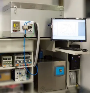
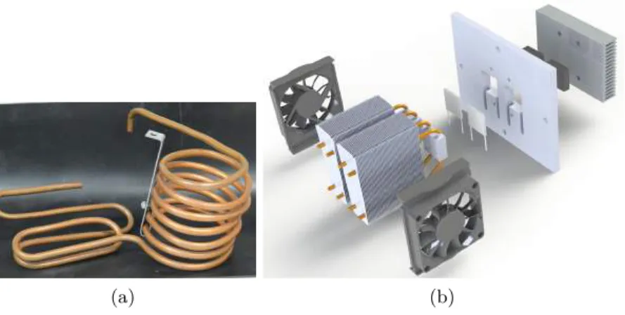
An exploded view of the regenerator ring with all its components is shown in the figure. A rendered image of the final setup of the experimental device is shown in Figure 10.

Magnetic circuit
The temperature of the liquid and the room temperature were maintained at 293 +− 1 K with a thermostatic bath and an air conditioning system, respectively. The dummy regenerator beds were placed directly between the pressure transmitters as shown in the figure. The virtual beds were filled with stainless steel balls approximately 0.5 mm in diameter.
Cold end flow distributor
EXPERIMENTAL ANALYSIS
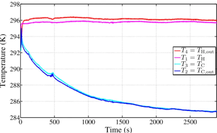
𝑇1: The temperature of the liquid entering the regenerator from the hot end during the hot-to-cold blow (hot blow). 𝑇2: The temperature of the liquid leaving the regenerator at the cold end during the hot-to-cold stroke. 𝑇4: The temperature of the liquid leaving the regenerator at the hot end during the cold-to-hot blow.
EXPERIMENTAL RESULTS
92 shows the behavior of the system temperature range (Δ𝑇sys) as a function of the regenerator temperature range (Δ𝑇reg) for the experiments presented in the figure. Behavior of the temperature range of the system (Δ𝑇sys) as a function of the temperature range of the regenerator (Δ𝑇reg) ) for the experiments in Fig. It is worth noting that the torque converter was installed on the motor shaft (Fig. 76), whose rotation frequency is the same as the operating frequency of the AMR.

PERFORMANCE EVALUATION RESULTS
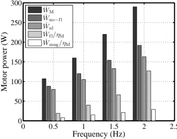
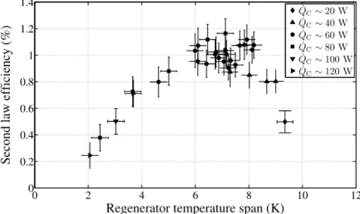
101 shows the results for the calculated 𝜂2ndas function of the regenerator temperature range for the experimental results presented in Fig. 102 shows the results of the calculated COP and 𝜂2ndas function of the time-averaged actual engine power, 𝑊˙ M, at different operating frequencies. This is probably related to the dependence of motor power on frequency (Fig. 99).
SUMMARY
PERFORMANCE ANALYSIS OF THE DTU MAGNETIC REFRIGERATOR
INTRODUCTION
EXPERIMENTAL WORK
The tests to determine the regenerator temperature span dependence on the hot reservoir temperature were carried out at the 400L/h volumetric flow rate (measured on the cold side). Alternatively, the tests to determine the regenerator temperature range as a function of the volumetric flow rate were performed at a hot reservoir temperature of approximately 297.7 K. This uncertainty is difficult to determine because it depends on many factors, such as the intrinsic uncertainties in the temperature sensors themselves and change in flow conditions due to wear of the sealing surfaces, parasitic losses and aging of the plastics and materials.

MODELING
- Numerical simulation
- Analysis of parasitic losses
Since the internal diameter of the flow head is quite large and is not subject to external conditions, it is assumed to be adiabatic. In the numerical model, the regenerator bed walls are treated as adiabatic, but in reality there will be heat transfer to the surroundings through the regenerator walls along the entire length of the regenerator. Therefore, heat losses in the regenerator beds were calculated by the integral of the thermal gradient along the regenerator bed.

PERFORMANCE METRICS
- Exergetic-equivalent cooling capacity
- Second-law efficiency
The internal thermodynamic losses associated with the refrigeration cycle are calculated based on the viscous power of the working fluid, 𝑊˙visc, through the layers of the regenerator, Eq. 𝑊˙visc+ ˙𝑊mag (6.8) Mechanical losses associated with liquid pumping, i.e. pump losses are calculated based on the liquid pumping power, 𝑊˙P, defined by Eq. The COPAMR is the COP of the actual AMR without the mechanical and electrical losses external to the regenerator, but inherent to the actual propulsion system.
RESULTS AND DISCUSSIONS .1 Parasitic losses
- Experimental results
- Hot reservoir temperature dependence
- Volumetric flow rate dependence
- Inputs Sensitivity
- Performance evaluation results .1 COP analysis
- Exergetic-equivalent cooling capacity
- Second law efficiency
110 and 111 show the results of COP, COPno−fl and COPAMR as a function of hot reservoir temperature and volumetric flow rate, respectively. The trend of 𝐸𝑥Q as a function of hot reservoir temperature resembles that reported in the literature (Russeket al., 2010). General and second law cycle efficiencies as a function of hot reservoir temperature and volumetric flow rate are shown in Fig.