Development of Control Strategies for the Joined-Wing Aircraft

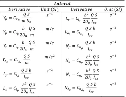
Change in lift coefficient due to deflection of control surfaces Rolling moment coefficient. Change in caused by the change in directional velocity Change in due to the deflection of the control surfaces Yaw moment coefficient.

Development of the Joined-Wing concept

Thesis motivation

Three different designs emerged from the aircraft manufacturers' competition, the high-aspect-ratio conventional wing, the flying wing, and the composite wing [8]. The Joined-Wing Sensorcraft configuration belongs to the Boeing aircraft and some work has been done by USAF partners building and testing smaller SensorCraft models [9].

Thesis objectives

An ambitious plan was proposed to the airlines, demanding new challenges: high endurance, outstanding aerodynamic performance, large payload capacity, power and cooling to support a next-generation intelligence, surveillance and reconnaissance (ISR) sensor. Conventional joined wing configurations always retain the vertical stabilizer; however, the strict requirements for long endurance and high aerodynamic performance led to this configuration.

Properties definitions

Multiple control surfaces that could be mounted in both the front and rear wings contributed to the feasibility of mixed control techniques on the SensorCraft. As a designation for the positive and negative direction of deflection of the control surfaces, downward deflection is defined as positive deflection and upward deflection is defined as negative deflection.

Thesis layout

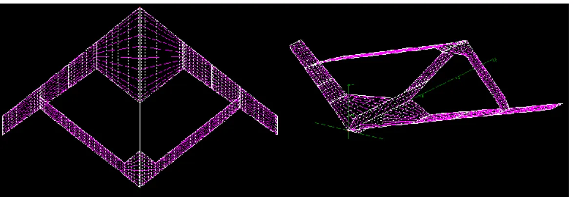
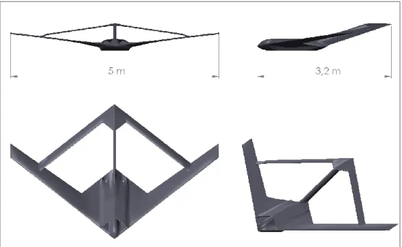
As previously mentioned, the Joined-Wing SensorCraft has a two-wing configuration in which the leading wing is positively dihedrally swept back to join the rear wing, which is anhedrally swept forward, creating a diamond shape that sweeps from above and forward views can be seen (figure 2.1). The fuselage is connected to the end of the rear wing by a tail beam, which provides better structural and aeroelastic responses of the wings during the SensorCraft flight.

Configuration and aircraft properties

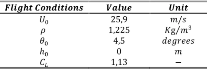
The flight condition parameters are given in Table 2.1, where is the forward speed of the aircraft and is the air density for the given reference altitude. Six control surfaces are located in the forward wing and the other four in the aft wing.

Control strategies in rudderless aircraft configurations

Differential thrust is achieved by creating a differential thrust between the engines, giving more power to one and less to the other, for example. Therefore, this third method will not be considered and only the first two methods will be analyzed.

Dynamics of flight

This theory essentially describes all motion variables in the equations of motion as having two components, a reference (or equilibrium) component and a dynamic (or disturbance) component as shown in the following expressions. The equations for , and are referred to as equations of longitudinal motion since they deal with all motions in the -plane.

State space representation of the equations of motion

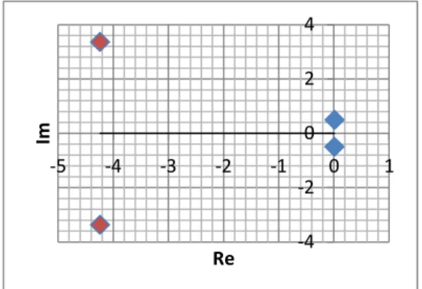
The results for longitudinal motion are detailed in Figure 4.2, which is the representation of the eigenvalues ​​in the Argand plane. In Table 4.2, the values ​​of the eigenvalues ​​are presented, as well as their correlation with the short period and the phugoid modes. The lateral movement was determined by the flight quality of the Dutch roll mode.

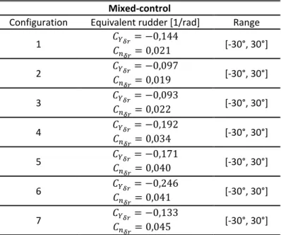
To achieve a negative yawing moment, the deflections of the control surfaces are the same, but in the left wing. The equations represent the stability coefficients and of the equivalent rudder for configuration 7 multiplied by the control surface. From Figure 5.5, the open loop of the lateral system has been shown to have an average performance in relation to the deflection of the ailerons.

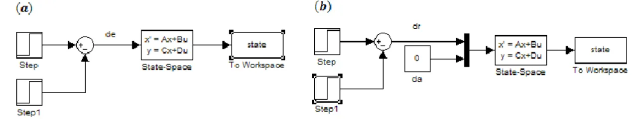
The time-space analysis of the close-loop system (feedback system) was simulated in the ® environment. A representative process of the Dutch role mode and its explanation is given in Figure I.4.

Determination of stability coefficients using

Stability coefficient estimation

Since stability coefficient estimation formulas are mostly available for conventional aircraft, various configurations must be adjusted to be used in such formulas. The value of obtained for SensorCraft was compared with values ​​for conventional aircraft in reference [16], and confirmed to be within their range of variation, which was.

Drag contributions

Since you do the calculations for an airfoil and for a wing surface, the drag coefficients are adjusted by different parameters. To solve this problem, the general equation of total aircraft drag was used, as described in equation (3.4).

Determination of the Parasitic Drag using XFOIL

After the curve is obtained, the stability coefficient of the parasitic drag versus the angle of deflection of control surface. 1) The position of the control surface hinge is the ratio of the chord where the control hinge is located.

Determination of the Induced Drag using AVL

For the sake of the example, in the worst case (outboard aileron maximum deflection), the difference between the values ​​of for the correct curve slope (taken at parabola minimum) and for the used curve slope is. Compared to the value of for the same deflection, that is, the variation is very small. Therefore, the errors allowed are small and the analysis can proceed with the approximation made for the curve slopes.

In addition, the allowable curve slopes above are bounded by the correct values ​​of the curve slope, so that the solutions will never exceed the actual limits.

Yaw coefficient results

As expected, the yaw moment coefficients will be strongly dependent on the direction of deflection, as can be verified in Table 3.6. Stability is a property of an equilibrium state, so the meaning of equilibrium must first be defined. Stability is the property of an aircraft to maintain the trimmed flight condition and for a given disturbance of forces and moments, it tends to restore the original condition.

The stability of an aircraft is divided into static and dynamic stability.

Static stability analysis

Since all SensorCraft stability coefficients have been fully described, it is now possible to proceed with the stability study. Static longitudinal stability is based on the analysis of the longitudinal properties of the aircraft described below. If an aircraft is longitudinally stable, a small increase in angle of attack will cause a change in the pitching moment, which decreases the angle of attack.

Describing which aerodynamic properties contribute to the static stability of the aircraft, the analysis is presented in Table 4.1.

Dynamic stability analysis

The dynamic stability of disturbed longitudinal motion is established from the knowledge of the eigenvalues ​​of the mode coefficient matrix presented in equation (2.79). In flight dynamics it is usual to factor the quadratic equation (4.2) into two quadratic factors corresponding to the short period and the phugoid mode:. 4.3) The first factor contains the eigenvalues ​​for the short period mode, where it represents the short period damping ratio and represents the short period frequency. The dynamic stability of perturbed lateral motion is established from the knowledge of the eigenvalues ​​of the mode coefficient matrix presented in equation (2.80).

In order to achieve the results of dynamic stability of transverse and longitudinal movements, the determinant in equation (4.1) was calculated using

Flying qualities evaluation

However, the overall flight quality of the longitudinal movement is the worse of the two modes. As with longitudinal motion, the overall quality of lateral motion is determined by the worst of the three lateral modes. Since the dutch roll mode has the worst flight quality level, the overall side movement flight quality is.

In summary, the longitudinal motion is unstable due to the phgoid mode, since the mode separation is respected and the short period mode is.

Configuration analysis of different control surface deflections

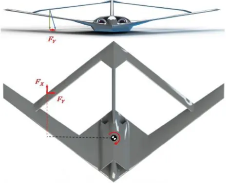
Therefore, there are many possible combinations of the control surfaces to achieve a required condition. As demonstrated in figure 4.5, the cancellation of vertical forces will cancel the roll moment and the lateral forces will act on the yaw moment of the SensorCraft. From figure 4.10 it appears that we can freely choose the direction of deflection of control surfaces in SensorCraft.

The speed braking control configurations analyzed are shown in the following figures and follow the same format as the previous configurations.

Equivalent control surface transformation

After determining the relationships between the control surfaces, the deflections can be replaced in the equations. From the control surfaces in the front wing, the inboard ailerons (C2) are chosen to maximize yaw and minimize roll by deflecting in the opposite direction to the elevators. As in the previous configurations, the equations represent the stability coefficients, and of the equivalent rudder of configuration 6, multiplied by the deflection of the control surface.

In the front wing, the flaps (C1), the inner and outer ailerons (C2 and C3) are represented by , and , respectively.

Aircraft open loop system

The time-space analysis of the open-loop system was tested in the multi-domain ® simulation environment. The open loop longitudinal system from figure 5.4 has an unstable response to elevators, as concluded in the previous chapter through the flight characteristics analysis. All lateral state variables are damped after the bars are disturbed and the system returns to equilibrium.

However, since the eigenvalue of the state variable is located at the origin, convergence is only ensured for larger values.

Control system design

In the previous figure, the size of the acquisition was first chosen for the solution that better stabilizes the Dutch role. Finally, the lateral movement due to the rudder deflection shown in figure 5.13 shows a very rapid convergence of the state variables, just after the disturbance in the control surface has ceased. Even the state variable has a fast convergence, which proves the effectiveness of the applied feedback in the Dutch role.

The root locus amplification results for the lateral configurations are shown in Table 5.6, as well as the eigenvalues ​​of each configuration.

Configurations results analysis

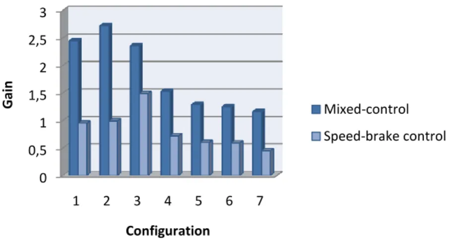
This analysis is easy to see in Figure 5.19, which represents the rate of convergence of the heading angle, and in the following graphic, which will highlight the results obtained for the gain values ​​of each configuration. As a result, it will be more difficult to perform an evaluation of the swing performance between multiple configurations. The loss of autonomy of the rolling movement of the aircraft does not justify their use.

In configuration 6, the addition of flaps cancels out the rolling moment produced by the elevators, allowing the elevators to make the largest contribution to the pitching moment.

Qualitative validation with the SensorCraft heuristic model

The flight test results were based on observing the aircraft's responses to the control inputs, and on the pilot's feedback. The stability parameter defines the behavior of the aircraft, after the rudder equivalent surface is applied. The comparison with a Joined-Wing heuristic model resulted in a qualitatively better yaw control for the speed brake configurations instead of the mixed control configurations.

8] Lucia D.J., ''The SensorCraft Configurations: A Non-Linear AeroServoElastic Challenge for Aviation'', 46th AIAA/ASME/ASCE/AHS/ASC Structures, Structural Dynamics & Materials Conference, Austin, Texas, April 2005. Figure I .5 represents the explanation of the roll mode and the appearance of its regenerative roll moment. The aircraft is considered to belong to one of the four classes shown in Table J.1 according to reference [12].