Development of a Guidance and Control Design Tool for Entry Space Vehicles with Different Lift-over-Drag Ratios

78 6.11 LowL/DRV on the Shuttle Entry Guidance algorithm in the drag speed plane: entry profile. 79 6.12 HighL/DRV on the Shuttle Entry Guidance algorithm in the drag speed plane: entry profile.

Context

Objective

Background

Approximate ballistic entry occurs when the L/D of the body is low, typically when L/D <0.5, which is the case of meteoroids, ICBMs or capsule-like vehicles, e.g. The Apollo Command Module (Apollo CM), Soyuz, or all re-entry vehicles (RVs) that have performed entry to Mars. The only existing example of successful lift-off entry is the Space Shuttle Orbiter, which uses its ability to generate significant lift force to distribute energy in a controlled manner during re-entry, while also being able to change trajectory her to reach the landing place safely. .

The re-entry problem

Entry dynamics

Furthermore, LandD are the aerodynamic rates of lift and drag force per unit mass, respectively, the rate of the gravity vector, and σ is the rib angle, which is used by the guidance and control (GC) system as the main variable of control. In this work, a coordinated motion of the vehicle is assumed, which implies a state of zero slip and zero lateral force.

Bounds and constraints

The slip angle is the angle between the velocities along the major and lateral axis of the vehicle. On the other hand, vehicle design is critical for determining the EIP and TAEM conditions, and for determining the reentry profile and associated limitations.

Impact of EIP conditions on the re-entry profile

The greater the speed of entry, the more sensitive is the capture of the vehicle in the atmosphere, and the heat flux and deceleration that the vehicle will suffer thereafter is necessarily greater. Regarding the dependence of FPA on entry velocity, the higher the entry velocity, the steeper the maximum FPA that still ensures capture.

Guidance in re-entry

The Guidance and Control function

However, the definition of the angle of attack is critical to maintain the dynamic balance and stability of the RV during reentry. The bank angle σ is thus the fundamental output parameter of the outer loop GC system.

Review of some guidance solutions

In a 3-DoF setting, the RV pose is not taken into account, meaning that the GC system is only applied to the outer loop dynamics of the RV tip mass motion. Because this generates a lateral deviation from the target, bank angle reversals are performed, changing the sign of the bank angle (note that the cosine function does not provide the sign of the bank angle), but its magnitude remains the same (to keep the angle of inclination). the vertical lift component as output by the control algorithm).

Overview of the work developed

This profile generation algorithm was tested using LQR control for reference tracking and further validated through Monte-Carlo tests. Therefore, the Apollo Entry Guide is now suitable for the wider capsule-like RV class, the Boat Entry Guide is suitable for the moderate L/D RV class and the enhanced E-Guide is suitable for the highL class /D.

Introduction

Since one of the axes is aligned with the RV velocity vector, the drag and lift forces can be written directly in this frame, along the X-axis and Z-axis respectively. This simplifies the writing of the equations of motion and provides better insight into the motion of the vehicle during reentry, which justifies why typically uses this frame of reference to develop management solutions.

Simulation

Equations of motion

This simplifies the writing of the equations of motion and provides more insight into the motion of the vehicle during re-entry, which justifies why this frame of reference is commonly used for the development of control solutions. the frame is not inertia: these are the Coriolis acceleration and the centripetal acceleration. Initial conditions for time t=t0, in the intrinsic reference frame, are written as 2.3) The initial and final conditions, written in the intrinsic reference frame definition, are translated and rotated internally to the ECEF reference frame and used to initialize and terminate the propagation of the equations of motion (2.1), which is done in the ECEF reference frame.

Atmospheric and aerodynamic parameters

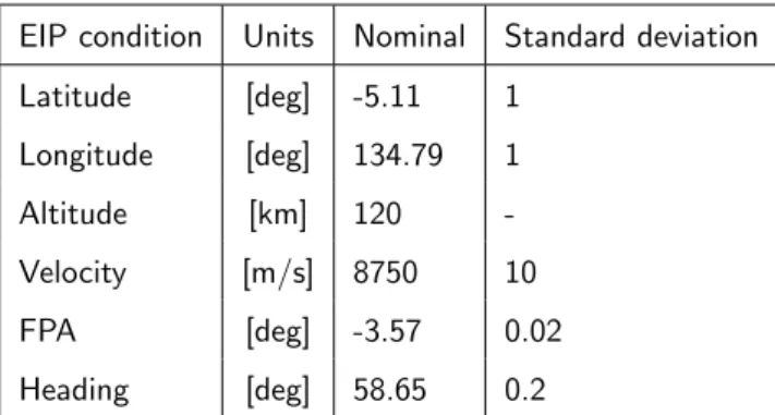
For the propagation of the equations of motion and for the termination of the propagation, the definition of the EIP and TAEM conditions is required.

Planet environment

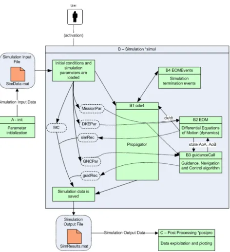
Simulator implementation

• Main function
• Initialization
• Simulation
• Monte-Carlo setting
• Result post-processing

GNC parameters, which are all the parameters related to the implemented guidance schemes (further discussed in chapters 3 and 6). While the propagation is performed in the ECEF reference frame, the intrinsic reference frame is used for the calculation of the aerodynamic variables, which are then converted to the ECEF reference frame.

Tests

Implementation test

Impact of EIP conditions and L/D in re-entry trajectory

As the entry velocity is reduced, the re-entry profile becomes smoother and the magnitude of the longitudinal oscillations is reduced (although this effect is more noticeable in the case of the shallower EIP FPA). The impact of the different RV aerodynamic characteristics in the re-entry profile is shown in Figure 2.13, where the EIP conditions are the same in all cases (Table 2.4).

Remarks

Introduction

Modelling the Shuttle Orbiter re-entry vehicle

The Shuttle Entry Guidance scheme

• The reference profile
• Reference angle of attack
• Controller
• Crossrange control

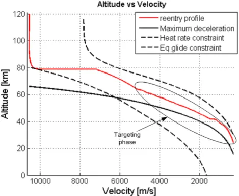
The reference profile [17] is shown in Figure 3.3, where five different phases of the entry profile and path restrictions are defined. The variation of the angle of incidence ∆αterm is thus added to prevent this deviation.

Implementation notes

Tabled equations

In this way, lateral movement of the RV is compensated from side to side. Finally, the third set of expressions shown in Table 3.3 is related to refreshing the reference profile, in case the predicted range differs from the expected range.

Prototyped functions

ShuttleGuidance.m Main function: perform the main calculations, call other subfunctions RangePrediction.m Calculate the range prediction assuming that the reference profile is followed NewProfile.m The drag velocity profile is updated depending on the range constraints RefProfile.m Reference profile values ​​are evaluated. LateralLogic.m The sign of the bank angle is determined depending on heading error gains.m The PID controller gains f1 andf2 are calculated.

Testing

From Figure 3.8 it is possible to conclude that the bank angle resulting from the current algorithm implementation closely matches the bank angle results in [17], while the bank turns occur at approximately the same speeds. However, it is clear that because the propagated dynamics is limited to 3-DoF (and not 6-DoF, as is the case with the results in [17]), there are discontinuities in the simulated bank angle output.

Generalization of the Shuttle Entry guidance

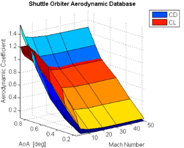
For the evaluation of these equations, the derivative of the drag coefficient is evaluated analytically to generalize the Shuttle guidance to other vehicles. In REACTIVE, the drag coefficient and its derivative are calculated using 3.13b) where α and M are the arbitrary order of the polynomial.

Remarks

In [17] it is proposed that CD0 C˙D0 approximates with. which uses a second-order polynomial to model the dependence of CD on angle of incidence α and an exponential relationship to model the dependence of CD on Mach number. To make this implementation more flexible, the CD approximation used in REACTIVE uses a combination of two polynomial terms of arbitrary order, one depending on the angle of incidence and the other on the Mach number.

Introduction

The implementation of these algorithms in REACTIVE consisted not only of consolidating the available algorithms, but also aimed to generalize the application of these algorithms (similarly to what was done in Chapter 3 regarding Shuttle Entry Guidance ) to generally low (in the case) of Apollo Entry Guidance) or high (in the case of Enhanced E-Guide) L/DRVs.

The Apollo prototypation

Apollo Commmand Module

Apollo Entry Guidance

These are used only to adjust the position and energy of the vehicle to the values ​​required for the activation of the aiming phase. The desired sdes range is determined by the navigation and targeting functions of the Apollo algorithm.

Apollo derivatives computation

Note that this maximum value is a constant, and that the argument of the arc cosfunction comes from the result of (4.2), in the final stage of the input guidance algorithm. To perform the generalization of the Apollo Guidance, in REACTIVE the F1, F2 and F3 derivatives are calculated analytically.

Highlift vehicle and guidance solution

Phoebus vehicle

This difference may be due to a mismatch in the atmospheric model and the aerodynamic model of the RV. It is important to note that generalizing the Apollo targeting approach to other capsule-like RVs requires that a reference entry profile associated with the RV be available.

Enhanced E-Guide

In the targeting phase, which is the last phase of the enhanced e-guide, the guidance scheme follows the reference profile to achieve the predefined TAEM conditions. A reference profile is generated offline and the system is linearly oriented with respect to this reference using energy as the independent variable.

Flexibilization of Enhanced E-Guide

Ultimately, REACTIVE's generalization of the enhanced e-guide can be seen as three independent guidance schemes that can be arbitrarily connected depending on the characteristics of the RV and the desired re-entry profile: altitude tracking with NDI, heat flux tracking with NDI, and onboard reference tracking profile.

Remarks

Introduction

To improve these results, another approach was developed, where the low-rank expression (5.2) is approximated by a polynomial depending on the velocity V, whose coefficients are determined through the method of least squares [40]. Regarding the rib angle, a three-degree-of-freedom σ(V) law is constructed, where two degrees of freedom are constrained by the initial and final conditions (TBVP boundaries) and the third is set so that the lower range requirement. is completed.

TBVP identification

Equations of motion

This relation is analytically integrated with respect to the velocity V and a constant rib angle solution is found. In this way, the reference profile generation (RPG) procedure ensures that the initial and final conditions, as well as the low range requirement, are met.

Boundaries

Approximate analytic bank angle solution

Obtaining the approximate analytical solution

Finally, the bank angle must also be assumed constant, which is a constraint on solving the problem, rather than a simplification, since the bank angle is a free control parameter. Note that it is possible to simplify (5.11) if we further assume that the FPA is also small enough so that sinγ≈0,cosγ≈1, which is the case most of the time.

Limits of validity

Expression (5.10) gives a relationship between downranges and slope angle σ, with speed as the independent variable. To write the slope angle in terms of downrange, inversion of this nonlinear relationship is required.

• General description
• Determination of the altitude and FPA profiles
• Downrange estimation using the Least Squares method
• Bank angle determination

For the estimation of the profiles, it is assumed that both (5.16) and (5.17) are only dependent on velocity, while the other variables appearing in the two expressions, e.g. The evaluation of equations (5.16) and (5.17) requires the estimation of the variables that appear in the right-hand side of the equations.

Implementation and tests

Implementation setting

In this way, a bank angle law that satisfies the downward criteria and initial / final conditions is determined. Finally, it is only necessary to generate the reference trajectory profile associated with the final bank angle law.

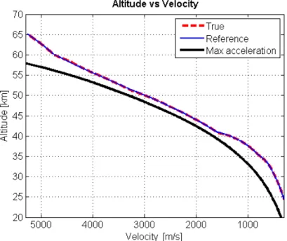
Nominal simulations

The pitch reference command shown in Figure 5.7 is followed with an average margin of error of 2 degrees. Figure 5.8 shows the trajectory of the vehicle, showing its accurate targeting capability in the nominal case.

Monte-carlo tests

Application: vehicle downrange capability

Remarks

Finally, the application of these guideline approaches for downside forecasting may be important for the initiation of the targeting phase. Prediction of the downward capability of the RV can be used instead, which will further improve the targeting results.

Introduction

REACTIVE tool integration

Hierarchical decomposition

This organization makes the addition of new vehicles and guidance schemes simple and flexible, requiring only to add an associated parameter database in the initialization function under the Setup folder, and create a function under the simulation folder that implements the desired guidance algorithm. In the same way, it is possible to add new atmospheric databases and planetary environments to the tool.

Entry vehicles & guidance schemes roundup

The parameters presented in Table 6.2, although relative to each specific motorhome, should be interpreted as being representative of the associated wider class of vehicles defined by the L/D ratio. Dhas on this parameter: The greater the L/D, the greater the downrange/crossrange capability of the RV.

Results

Guidance schemes with associated vehicle class

In general, the obtained results show that the integration and consolidation of the algorithms was successful. REACTIVE is thus able to implement implemented control schemes on any vehicles of the connected L/D class.

L/D class study

It is only suitable for RVs with 1.8< L/D <2.5 as the L/Dmargin is critical for tracking the reference altitude in the first stage of NDI. For L/D below this threshold, it was verified that the RV was unable to track the reference altitude and exited the atmosphere.

Mixing guidance schemes and associated vehicle class

For higher L/Ds, a problem with the LQR controller starts to show in the final stage. This is because the controller's planned gains are not sufficient for the new vehicle configuration, as it is different from the one used in their determination.

Extension to Mars scenario

Clearly, as documented in Figure 6.10 for the L/D= 2.5 case, there is an unwanted rocking motion below V = 5 km/s.

Remarks

Conclusions

Examples of this are the NDI approach to the Enhanced E-Guide algorithm and promising approaches such as the predictive control model technique for re-entry [39], or dynamic controller synthesis using robust Control Theory [30]. Other hot topics, such as neural networks [5, 46], line construction or reinforcement learning [7], may also be viable solutions for RVs with significant L/D in the future, but they still need to be tried in other less demanding contexts.

Future work

Crossrange control in the profile generation procedure

Evolution of REACTIVE

Branco. High Lift Above Drag Reentry - Earth Reentry Guidance Techniques for Human Missions. Air heating path and environment development and sensitivity analysis for capsule vehicles. American Institute of Aeronautics and Astronautics, 2005.