Development of Software for Antenna Analysis and Design using FDTD

TRAMITAÇÃO DE DISSERTAÇÃO/PROJECTO

INFORMAÇÃO A INTRODUZIR NO SISTEMA FÉNIX

CONFIDENCIALIDADE

ESTRUTURA E FORMATO DA DISSERTAÇÃO

Impressão da Dissertação

Capa e Lombada

Equações e Expressões

Tabelas e Figuras

ESTRUTURA DO RESUMO ALARGADO

ESTRUTURA DO CD

MODELO DE CAPA E LOMBADA

MODELO DE CAPA DE CD

FICHA DE HOMOLOGAÇÃO de JÚRI

CONTEÚDO DE identificacao.pdf

DECLARAÇÃO RESPEITANTE À DIVULGAÇÃO DA DISSERTAÇÃO

EXEMPLO DE DECLARAÇÃO DE CONFIDENCIALIDADE

Brief historical background of Computational Electromagnetics

In fact, it can be said that much of the technological progress made in the last fifty years would not have been possible without the ability to solve Maxwell's equations quickly and accurately at large scales. After 1960, with the availability of programmable electronic digital computers, the first computational approaches for Maxwell's equations appeared.

Currently available software

Objectives of this work

Because flexibility is an essential requirement, the tool will be modular, making it relatively easy to add new functionalities or even incorporate part of the tool into another program. Having stated the objectives of this work and their motivation, it is now necessary to justify the choice of the FDTD technique.

Why FDTD?

• Techniques in Computational Electromagnetics
• FDTD advantages

The main reasons for this choice were the author's mastery of the language, the ability to use a high-level scene-based API for 3D graphics (Java 3D) [5][6] and the seamless portability of the software between different types of software. machines and operating systems. Nevertheless, since the program has a modular structure, some modules can easily be rewritten in another language, as could be the case if one wanted to optimize the computation-intensive part of the code by writing it in a native language.

List of implemented features

This chapter presents the fundamentals of the finite difference time-domain method and the derivation of the algorithm used in this work. For the derivation of the FDTD algorithm used in this work, only diagonal tensors will be considered, that is, with the following matrix representations.

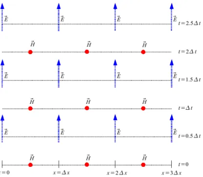
The Yee Algorithm

• The Yee cell and the leapfrogging scheme
• Discretization of Maxwell’s Equations using the Yee algorithm
• Computer Implementation

Based on this lattice scheme, Yee discretized a version of the set of equations (2.15) and (2.16) specified for lossless isotropic media using central difference terms, for both space and time derivatives. By using this notation, a numerical approximation of the set of equations (2.15) and (2.16) can now be obtained.

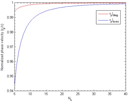
Numerical Dispersion

• Derivation of the numerical dispersion relation for three-dimensional wave propagation 15

Although the error in the numerical phase velocity relative to the theoretical value can be made reasonably small with at least ten cells per wavelength, it is also important to take into account the anisotropy of the phase velocity. In such cases, the numerical errors are not due to numerical dispersion, but mainly to differences between the mesh version of the structure and its actual geometry.

Numerical Stability

• The Courant stability criterion
• Other potential sources of instability

The Courant stability criterion sets an upper bound for the time step to achieve a stable simulation. For the augmentation algorithms used in this work that tend to be unstable, a stability criterion or empirical rule will be presented in the respective section.

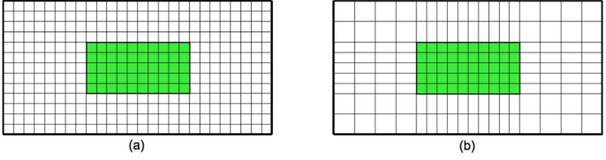
Extension to non-uniform Cartesian meshes

• Benefits of non-uniform meshes
• Required modifications to the algorithm
• Numerical accuracy and stability for non-uniform FDTD

As can be seen in fig. 2.5(b), a non-uniform mesh can adapt to the boundaries of both shapes, providing a better discretization of the geometry of the problem. Nevertheless, semi-analytical/semi-empirical criteria exist for the selection of time step ∆t and mesh characteristics that have enabled many successful engineering applications using non-uniform meshes.

Introduction

For this reason, the UPML formulation of PML was chosen for implementation in the developed software. Before describing UPML in detail in Section 3.3, an overview of B´erenger PML will be presented in Section 3.2.

B´ erenger’s Split-Field PML

3.1, for practical purposes the PML medium must be backed by PEC walls since the PML cannot extend to infinity. However, when applied to a numerical algorithm, a sharp variation of conductivity between the main computational domain and the PML medium gives rise to significant numerical reflections. Thus, to mitigate these reflections, the conductivity inside the PML must be gradually increased from zero at the interface to a value σm near the PEC walls.

Uniaxial PML

• UPML Formulation
• Theoretical and Practical Performance of the UPML
• Application to a Three-Dimensional Problem Space
• Implementation in FDTD
• Computer Implementation
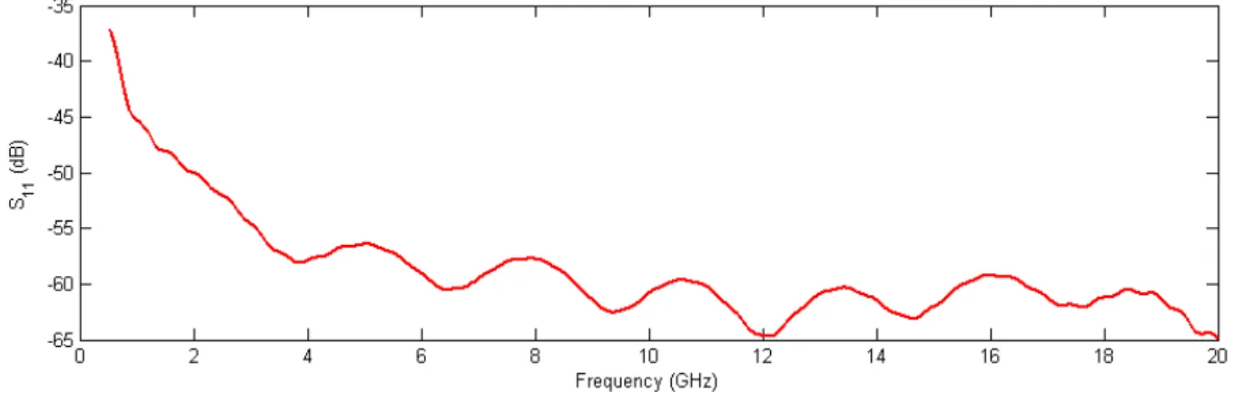
• UPML validation

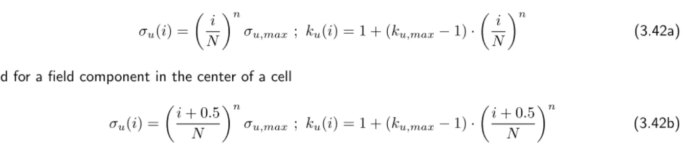
The computer implementation of the UPML update equations is very similar to that presented in Section 2.2.3 and therefore the update equations and coefficients for all field components are presented in Appendix D. It is also important to mention that in Discretized UPML the values ​​of ku and σu, where u=x,y,z, must be chosen according to the position of the field component within the UPML. The point source excited the Ex component of the (6,6,6) cell with a Gaussian signal having a -20 dB bandwidth of 2 GHz and the Exfield was measured in the (6,12,6) cell, which was side by side with UPML layers.

Thin-wire model

Applying Faraday's law to the contour C gives which can be converted to the following special time step ratio for Hy|i+1. The thin-wire model was implemented in the developed software simply by using specific time step ratios for the H-field loop components directly adjacent to the wire as shown in the figure. It is important to note that the other field components, namely the radial components of the electric field, are updated with standard time step relations, although special relations could also be derived for them.

Effective material parameters

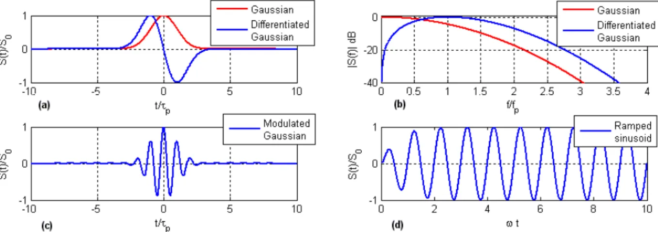
This physical consideration contradicts the previous assumption that the field is constant on both sides of the interface. Therefore, to explore this advantage, the signal used for excitation must have significant spectral content in the frequency band of interest. Finally, for those situations where the user really wants to analyze the behavior of the antenna at a single frequencyfc, a skewed sine excitation is included in the software, i.e. shape signal.

Point Source

Resistive voltage source

• Model description
• Calculation of Impedance and S parameters

The transmission line is excited at the index ko = ksource0 by adding the value of the excitation signal Vexc(t) to the voltage value already present on the line, corresponding to the following update relation. Vexc|n+1 (5.8) which corresponds to a soft source that generates voltage and current waves propagating both to the left and to the right of the excitation point. The coupling between the FDTD grid and the virtual transmission line is performed by assigning the current calculated from the local magnetic field values ​​to the current at the end of the transmission line, I|k0.

Simple Waveguide Source

• Model description
• Calculation of S parameters

The field distribution measured at the end of the line after the preliminary FDTD run is shown in Fig. It is important to note that in (5.18) both the characteristic impedance of the line and the incident field distribution are normalized to 1. The normalization of the incident field distribution is done using the inner product defined in (5.17).

Frequency-Domain Transformation

• Analytical expressions for the transformation
• Calculation of the equivalent M ¯ S and J ¯ S currents
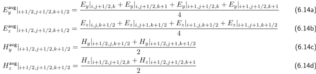
• Averaging of the E ~ and H ~ fields on the virtual surface

Assuming that the E and H field components used for the transformation are located at the center of the Yee cells, as shown in Fig. During the simulation and structure setup phase, the user specifies both the simulation parameters and the characteristics of the structure to analyze. Frequenciesatfminandfmaxw will also determine the bandwidth of the excitation signal (which is, by default, a Gaussian pulse), as discussed in section 5.1;.

Spatial Discretization Algorithm

To more clearly explain how the spatial discretization algorithm meets the foregoing requirements, the description of the discretization procedure for the non-uniform case will be accompanied by an example. The value chosen for Ris 1.3, which is the default value used in the mesh generation algorithm of the developed software. As can be observed, the mesh lines are aligned with the boundaries of the geometry, with the mesh resolution close to Dmax = 30.

Material Mapping Algorithm

7.4(a), which represents a two-dimensional view of the Cartesian mesh resulting from the discretization, using the algorithm described in the previous section, of a component consisting of three overlapping cylindrical structures, similar to a coaxial cable. For this reason, the algorithm will ignore structures for which this number is odd, displaying a message warning the user that the problem has occurred. 7.5(a) corresponds to the case of the coaxial cable, Fig. 7.5(b) shows a cylindrical waveguide, which was achieved by reducing the priority of structure S2 and changing the material of structure S1 in vacuum.

Monopole Antenna on a Conducting Box

Microstrip Patch Antenna

Since no experimental field results were available for this antenna, a qualitative comparison between the 3D radiation patterns for 7.55 GHz calculated with the developed software and CST Microwave StudioR is shown in Fig. This comparison essentially serves to demonstrate the software's ability to create three-dimensional radiation patterns. As can be seen, the patterns have a similar shape and there is little difference between the maximum directivity values: 7.957 dBi for CST and 7.943 dBi for the developed software.

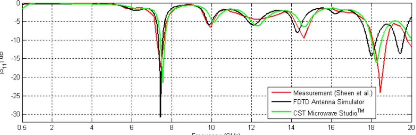
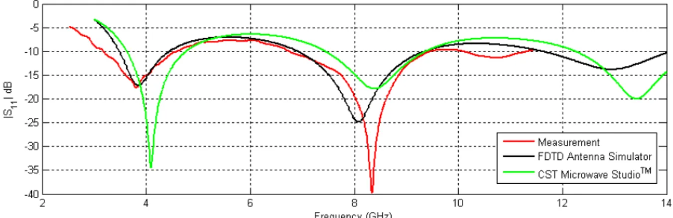
UWB Antenna

A 10-cell thick UPML layer was placed on the domain boundaries, and the time step used for the simulation was ∆t = 0.223 ps. The results can be considered relatively good, considering that the largest differences occur at the angles corresponding to the area where the coaxial cable was installed. The latter must also be taken into account when comparing measured and calculated radiation patterns.

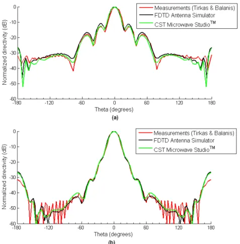
Pyramidal Horn Antenna

As already mentioned, great emphasis was placed on the generality and expandability of the developed software. However, it is important to note that the selection of Java as the main programming language does not in any way exclude the possibility of using other languages, namely C/C++ or Fortran, to implement the numerically intensive parts of the code. The techniques introduced by Dey and Mittra [46, 47] are known to produce good results and are relatively easy to implement in the developed software, by making some changes in the material mapping phase of the mesh generation algorithm;

Backward-differences approximation to the first derivative

Central-differences approximation to the first derivative

Central-differences approximation to the second derivative

Equation (B.7) shows that for a medium without conductivity, i.e. with σxx=σyy =σzz= 0, the time derivative of the net electric flux leaving the Yee cell equals zero, which means that, assuming zero initial conditions, this flux never deviates from zero and there is no free charge in the Yee cells. However, when there are currents in the computational domain, either due to non-zero conductance or excitation current, Yee cells implicitly store charge and capacitance between adjacent cells has been shown to exist [48]. The proof of verification of Gauss's law (2.4) can be done by analogy with the procedure used for (2.3), using the continuity equation for equivalent magnetic fluxes and charges.

Three-Dimensional FDTD Update Algorithm with the UPML

This appendix presents the field updating relations and coefficients used for the implementation of the UPML absorbing boundary in the developed software.

Update equations for the H-field

To illustrate this technique, consider a possible discretization of the microstrip line of Figure. This example illustrates the applicability of the software to the analysis of microstrip circuit components. The metal parts of the device were all interlocked as thin metallizations, as described in Appendix E.

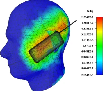
SAR Calculation

• Return loss of the line-fed rectangular patch antenna
• Three-dimensional radiation patterns for the line-fed rectangular patch antenna calculated using
• Geometry of the beveled planar monopole antenna and feed region
• Detail of the feed region and placement of the excitation source
• Return loss of the beveled monopole antenna
• Calculated x-z radiation pattern for the beveled monopole antenna at 8.5 GHz
• Calculated y-z radiation pattern for the beveled monopole antenna at 8.5 GHz
• Calculated x-y radiation pattern for the beveled monopole antenna at 8.5 GHz
• Geometry of the pyramidal horn antenna and detail of the mesh used in its simulation
• Directivity of the pyramidal horn at 10.1 GHz: (a) E-plane pattern, (b) H-plane pattern
• Calculated return loss of the pyramidal horn antenna

Mittra, “A technique to improve the accuracy of the nonuniform finite-difference time-domain algorithm,” IEEE Trans. Mur, “Absorbing boundary conditions for the finite-difference approximation of the time-domain electromagnetic-field equations,” IEEE Transactions on Electromagnetic Compatibility, vol. Balanis, "Finite-Difference Time-Domain Method for Antenna Radiation," IEEE Transactions on Antennas and Propagation, vol.

Geometry of the microstrip line used to illustrate the technique for modeling thin metalizations. 92

Geometry of the low-pass filter

Return loss of the low-pass filter

Insertion loss of the low-pass filter

Geometry of the SAR calculation problem.(a) Perspective view of the SAM and cell phone. (b)

Three-dimensional SAR plot for the CENELEC 50361 SAM phantom head

Illustration of the SAM phantom head’s effect on the radiation pattern (directivity) of the