Education Policy - CPS/FGV

Hgxfdwlrq Srolf|

Mdphv M1 Khfnpdq

Wkh Xqlyhuvlw| ri Fklfdjr dqg Xqlyhuvlw| Froohjh Orqgrq

Ixqgdêær Jhwxolr Ydujdv

Ulr Gh Mdqhlur/ Qryhpehu 5338

• In their edited book “What’s the Good of Education”

Stephen Machin and Anna Vignoles write

• “. . . Gary Becker [1964] presents an analytical framework to explain why individuals invest in education and train- ing in a manner analogous to investment in physical cap- ital. The resulting human capital theory is still the basis for research in the economics of education field today. . . ”

and

• “much of the progress that has been made in the eco- nomics of education field since the pioneering days of the 1960s and 1970s, and this certainly applies to its recent rejuvenation amongst economists, has been in terms of the quality of the empirical evidence available (and the techniques used to obtain that evidence) rather than in terms of theoretical developments”

• Similar sentiments are expressed by other labor econo- mists regarding the Mincer (1974) earnings function–

another product of the 1960s and 1970s.

• It is widely viewed as an enduring empirical and theo- retical success with universal application and is one of the most widely estimated empirical relationships in all of economics.

• The widely shared point of view that the economics of education is a settled area is reminiscent of late 19th cen- tury physics just before X rays, radioactivity, relativity and quantum mechanics revolutionized the field.

• In my short lecture today, I want to describe the consid- erable theoretical and empirical developments that have appeared in the past 15 years that are fundamentally changing the economics of education even if they have not yet changed the practice of most of the people work- ing in the field.

• For specificity, let me focus on progress in estimating returns to schooling and its implications for educational

• If the economics of education is a “settled” area, there are many unsettling empirical puzzles that the received theory cannot explain.

• Foremost among these is why the “returns” (read “Min- cer returns”) are so high compared to other investments.

• Why are not more people taking schooling if it is such a profitable investment?

• Exacerbating this is the sluggish enrollment response of recent cohorts to increases in returns over the past 20 years.

• Why is money left on the table?

• Why are enrollment rates not higher?

0 10 20 30 40 50 60 70 80

% Participating

Figure 1

Schooling Participation Rates by Year of Birth: Data from CPS 2000

A. Whites

3HUFHQWDJH

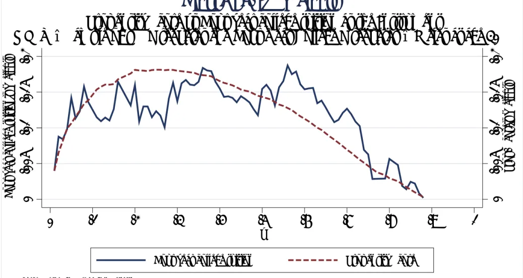
A. Share of High School Dropouts in the United States, 1971-1999

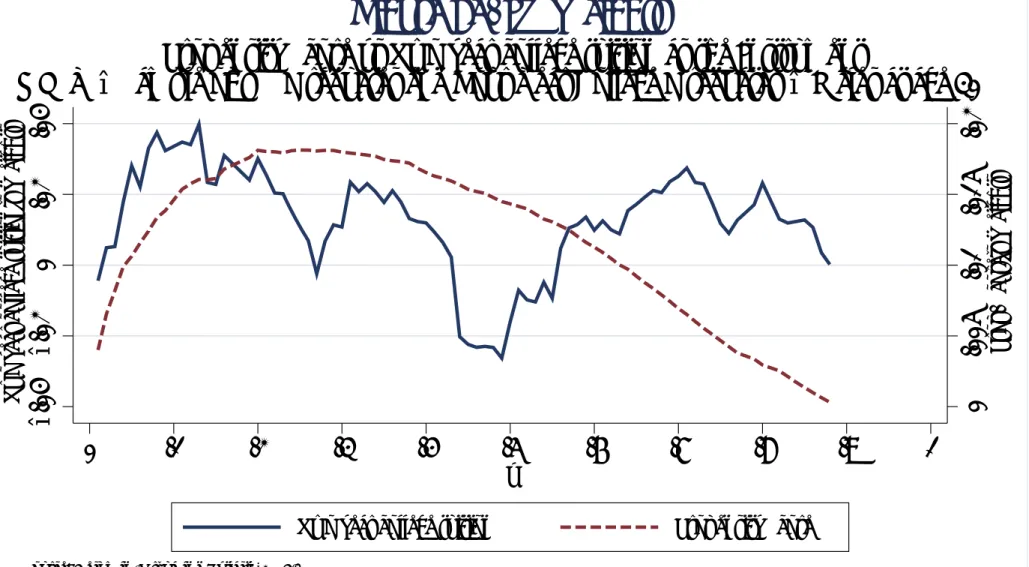
Figure 2

Educational Statistics by Category Over Time

724 QUARTERLY JOURNAL OF ECONOMICS

Figure 3

Central Tool Used to Estimate “Returns”

• Mincer equation:

ln[\ (v> {)] = + _vv + ₀{ + ₁{² + % (1) v schooling; _v “rate of return”

The Compensating Dierences Version

• Let \ (v) represent the annual earnings of an individual with v years of education

• u be an externally determined interest rate

• W the length of working life

• Y (v) = \ (v) R _W

v h^3uwgw = ^{\ (v)}_u (h^3uv h^3uW)= ln \ (v)

as W<" = ln \ (0) + uv + ln((1 h^3uW )@(1 h^3u(W3v)))= ln \ (v) = ln \ (0) + uv

The Accounting-Identity Model

ln \ (v_l> {_l) = _l + _vlv_l + _0l{_l + _1l{²_l + %_l=

• Accounting identity model

1. Allows for heterogeneity among persons (assumes _vl, independent of v_l but see Mincer, 1993)

2. Estimates an ex post average rate of return

3. Strong evidence against the parallelism in experi- ence assumed by this model

4. Ex post rates of returns derived from the model are very misleading compared to rates of return derived from IRR calculations applied to cross sections.

This is intended to approximate the internal rate of return for schooling level v₁ versus v₂, u_L(v₁> v₂), which solves

W(Zv₁)3v₁ 0

(1 )h^3uL({+v1)\ (v₁> {)g{

v₁

Z

0

yh^3uL}g}

=

W(Zv₂)3v₂ 0

(1 )h^3uL({+v2)\ (v₂> {)g{

v₂

Z

0

yh^3uL}g}= (2)

u_L will equal the Mincer coe!cient on schooling if

1. Parallelism over experience across schooling categories (\ (v> {) = (v)*({))

2. Linearity of log earnings in schooling ((v) = (0)h^vv) 3. No tuition and psychic costs (y = 0)

4. No taxes ( = 0)

5. Equal working-lives irrespective of years of schooling (W ⁰(v) = 1).

Wdeoh 4d= Lqwhuqdo Udwhv ri Uhwxuq iru Zklwh Phq= Hduqlqjv Ixqfwlrq Dvvxpswlrqv +Vshflfdwlrqv Dvvxph Zrun Olyhv ri 7: \hduv,

Vfkrrolqj Frpsdulvrqv

90; ;043 43045 45047 45049 47049

4<73 Plqfhu Vshflfdwlrq 46 46 46 46 46 46

Uhod{ O lqhdulw| lq V 49 47 48 43 48 54

Uhod{ O lqhdulw| lq V ) Txdg1 lq H{s1 49 47 4: 43 48 53

Uhod{ Olq1 lq V ) Sdudooholvp 45 47 57 44 4; 59

4<83 Plqfhu Vshflfdwlrq 44 44 44 44 44 44

Uhod{ Olqhdulw| lq V 46 46 4; 3 ; 49

Uhod{ Olqhdulw| lq V ) Txdg1 lq H{s1 47 45 49 6 ; 47 Uhod{ Olqhdulw| lq V ) Sdudooholvp 59 5; 5; 6 ; 4<

4<93 Plqfhu Vshflfdwlrq 45 45 45 45 45 45

Uhod{ Olqhdulw| lq V < : 55 9 46 54

Uhod{ Olqhdulw| lq V ) Txdg1 lq H{s1 43 < 4: ; 45 4:

Uhod{ Olqhdulw| lq V ) Sdudooholvp 56 5< 66 : 46 58 Qrwhv= Gdwd wdnhq iurp 4<730<3 Ghfhqqldo Fhqvxvhv1 Lq 4<<3/ frpsdulvrqv ri 9 yv1 ; dqg ; yv1 43 fdqqrw eh pdgh jlyhq gdwd uhvwulfwlrqv1 Wkhuhiruh/ wkrvh froxpqv uhsruw fdofxodwlrqv

Wdeoh 4e= Lqwhuqdo Udwhv ri Uhwxuq iru Zklwh Phq= Hduqlqjv Ixqfwlrq Dvvxpswlrqv +Vshflfdwlrqv Dvvxph Zrun Olyhv ri 7: \hduv,

Vfkrrolqj Frpsdulvrqv

90; ;043 43045 45047 45049 47049

4<:3 Plqfhu Vshflfdwlrq 46 46 46 46 46 46

Uhod{ Olqhdulw| lq V 5 6 63 9 46 53

Uhod{ O lqhdulw| lq V ) Txdg1 lq H{s1 8 : 53 43 46 4:

Uhod{ Olqhdulw| lq V ) Sdudooholvp 4: 5< 66 : 46 57

4<;3 Plqfhu Vshflfdwlrq 44 44 44 44 44 44

Uhod{ Olqhdulw| lq V 6 044 69 8 44 4;

Uhod{ Olqhdulw| lq V ) Txdg1 lq H{s1 7 07 5; 9 44 49 Uhod{ Olqhdulw| lq V ) Sdudooholvp 49 99 78 8 44 54

4<<3 Plqfhu Vshflfdwlrq 47 47 47 47 47 47

Uhod{ Olqhdulw| lq V 0: 0: 6< : 48 57

Uhod{ O lqhdulw| lq V ) Txdg1 lq H{s1 06 06 63 43 48 53 Uhod{ Olqhdulw| lq V ) Sdudooholvp 53 53 83 43 49 59 Qrwhv= Gdwd wdnhq iurp 4<730<3 Ghfhqqldo Fhqvxvhv1 Lq 4<<3/ frpsdulvrqv ri 9 yv1 ; dqg ; yv1 43 fdqqrw eh pdgh jlyhq gdwd uhvwulfwlrqv1 Wkhuhiruh/ wkrvh froxpqv uhsruw fdofxodwlrqv edvhg rq d frpsdulvrq ri 9 dqg 43 |hduv ri vfkrrolqj1 Vhh Dsshqgl{ E iru gdwd ghvfulswlrq1

• Nonlinearities in earnings function with respect to school- ing greatly aect computed ex post rates of return.

• Linearity of log earnings in schooling is rejected in most statistical tests.

• Linearity of not natural for another reason

• There are many educational credentials that are not part of regular schooling

1. GED (20% of high school graduates)

2. Vocational Training (graduates 40% of non-college students)

• So as educational choices proliferate, the Mincer model is less appropriate for explaining a broad portfolio of ed- ucational and skill enhancement courses.

• Can compute rates of return for these programs.

• Cannot be squeezed into the Mincer straightjacket.

• Years in school are not the same as investment.

Cross Section Bias

• Synthetic cohort approach is widely used

• Assumes cross sections are reliable guides to what life cycles will be

• Mincer showed that it was not a bad assumption for US data circa 1960

• It’s a poor assumption for the modern labor market

• Estimates from recent cross sections biased by cohort ef- fects (MaCurdy-Mroz, 1995; Card and Lemieux, 2001).

• Convention followed by Becker (1964)—Hanoch (1966) used to compute rates of return assumed that earnings in col- lege oset tuition costs.

• Implicit assumption in the literature was a version of ra- tional expectations in which agents use earnings of people at older ages to forecast their own earnings.

• But nonstationarity of the economic environment in the past 30 years and cohort eects makes this a bad ap- proach as we have just seen.

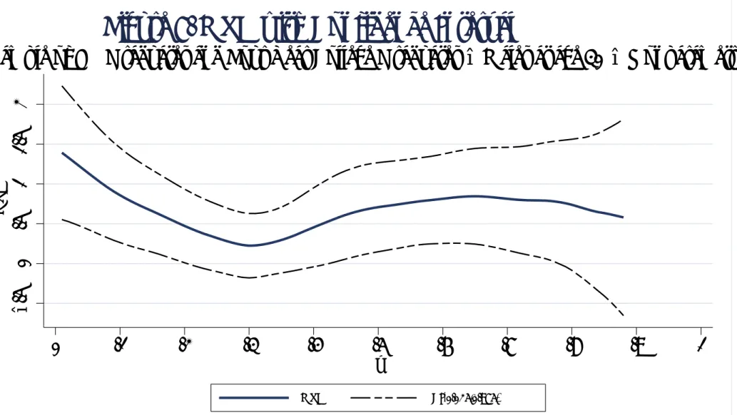
(KIWTG4+44HQTXU;GCTUQH'FWECVKQPHQT9JKVG/GPŦ %25

+44

ETQUUŦUGEVKQP EQJQTV

Uncertainty

• Conventional literature in the economics of education ignores uncertainty.

• Alternatively, gives an ex post analysis.

• It was developed in the 1960s when the economics of uncertainty was still being developed.

• Sequential revelation of information not incorporated into the basic theory.

• It also assumed that costs (psychic and tuition costs) were “negligible” (equation 2).

• Ad hoc ways to deal with uncertainty

1. People put themselves at the mean of the residual (H (%_l) = 0)

or

2. Take expectations of future earnings (mean of future income)

3. Choice of expectations assumption aects estimates of return

• Manski (1992,1993) gives some examples of how alterna- tive expectation formation assumptions aect estimates

• Suppose that agents base their expectations of future earnings at dierent schooling levels on the mean earn- ings profiles for each schooling level, or on H(\ |v> {).

In this case, the estimator of the ex ante rate of return is given by the root of

XW {=0

H(\ (v + m> {)|v> {)

(1 + ˆu_L)^v+m+{ (3)

XW {=0

H(\ (v> {)|v> {) (1 + ˆu_L)^v+{

Xm {=1

y

(1 + ˆu_L)^v+{ = 0=

If y = 0 and Mincer’s assumptions hold, this formula special- izes to

h^vm (1 + ˆu_L)^m

XW {=0

h^0{+1{2H(h^%(v+m>{)|v> {) (1 + ˆu_L)^{

=

XW {=0

h^0{+1{2H(h^%(v>{)|v> {) (1 + ˆu_L)^{ =

Wdeoh 5= Lqwhuqdo Udwhv ri Uhwxuq iru Zklwh Phq=

Uhvlgxdo Dgmxvwphqw

+Jhqhudo Qrq0Sdudphwulf Vshflfdwlrq

Dffrxqwlqj iru Wxlwlrq dqg Surjuhvvlyh Wd{hv, Vfkrrolqj Frpsdulvrqv

90; ;043 43045 45047 45049 47049

4<73 Xqdgmxvwhg 45 47 57 ; 48 54

Dgmxvwhg 5 5 ; < 46 49

4<83 Xqdgmxvwhg 58 59 59 6 : 48

Dgmxvwhg 4: 4< 47 8 ; 47

4<93 Xqdgmxvwhg 54 5: 5< 9 43 4<

Dgmxvwhg 46 4< 49 : 44 49

4<:3 Xqdgmxvwhg 49 5: 5< 8 43 4;

Dgmxvwhg 44 4; 49 9 43 49

4<;3 Xqdgmxvwhg 47 97 74 7 ; 48

Dgmxvwhg < 5; 57 8 ; 46

4<<3 Xqdgmxvwhg 4< 4< 7: ; 45 4;

Dgmxvwhg 44 44 64 ; 45 4:

Qrwhv= Gdwd wdnhq iurp 4<730<3 Ghfhqqldo Fhqvxvhv1 Lq 4<<3/ frpsdulvrqv ri 9 yv1 ; dqg ; yv1 43 fdqqrw eh pdgh jlyhq gdwd uhvwulfwlrqv1 Wkhuhiruh/ wkrvh froxpqv uhsruw fdofxodwlrqv edvhg rq d frpsdulvrq ri 9 dqg 43 |hduv ri vfkrrolqj1 Vhh glvfxvvlrq lq wh{w dqg Dsshqgl{ E

• But the open question is what is the correct information set? These adjustments are ad hoc.

• Dominitz-Manski (1996); Manski (2004) use surveys to elicit expectations.

• Raises a whole set of issues of what survey responses actually elicit.

• A basic issue in accounting for uncertainty is determining what it is that agents act on, what is in their information set.

• Will return to this.

Option Values

• Sequential resolution of uncertainty creates option val- ues.

• So does non-linearity of earnings in terms of schooling.

• This changes the way we think about the rate of return and is an important theoretical development.

Dynamic Sequential Model With Option Value:

• Uncertainty about net earnings conditional on v, so that actual lifetime earnings for someone with v years of school are

\_v =

" _W X

{=0

(1 + u)^3{\ (v> {)

# _v= _v is a one time, schooling-specific shock.

• Assume H_v31(_v) = 1

\¯_v = H_v31(\_v)=

Decision problem for a person with v years of schooling given the sequential revelation of information:

Complete another year of schooling if

\_v H_v(Y_v+1) 1 + u = Value of schooling level v, Y_v

Y_v = max

½

\_v> H_v(Y_v+1) 1 + u

¾

for v ? V=¯

At the maximum schooling level, V¯, after all information is revealed, YV¯ = \V¯ = ¯\V¯V¯=

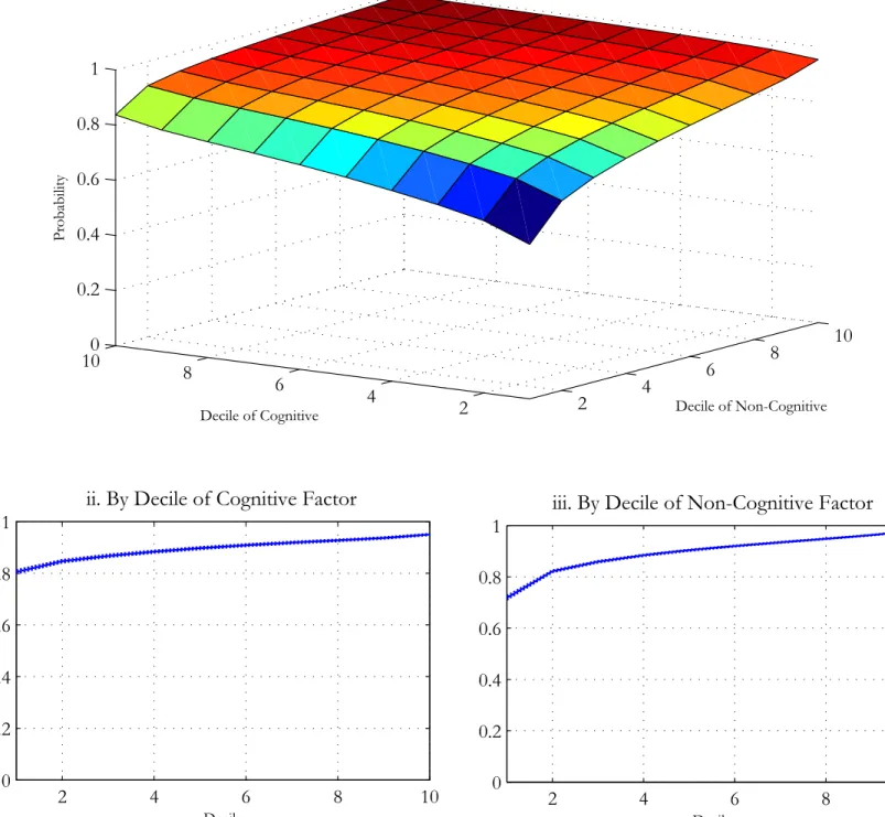
Probability of going from school level v to v + 1 : s_v+1>v = S u

μ

_v H_v(Y_v+1) (1 + u) ¯\_v

¶

>

H_v(Y_v+1) may depend on _v because it enters the agent’s infor- mation set.

The average earnings of a person who stops at schooling level v are

\¯_vH_v31 μ

_v|_v A H_v(Y_v+1) (1 + u) ¯\_v

¶

= (4)

Expected value of schooling level v as perceived at current schooling v 1 is:

H_v31(Y_v) = (1 s_v+1>v) ¯\_vH_v31 μ

_v|_v A H_v(Y_v+1) (1 + u) ¯\_v

¶

| {z }

+s_v+1>v

μH_v31(Y_v+1) 1 + u

¶

=

The first component is the direct return. The second compo- nent arises from the option to go on to higher levels of school- ing.

• Option value of schooling v

R_v>v31 = H_v31 [Y_v \_v] =

• Option values are non-negative for all schooling levels, since Y_v \_v for all v.

• Ex ante rate of return to schooling v as perceived at the end of stage v 1 is

U_v>v31 = H_v31(Y_v) \_v31

\_v31 = (5)

• No direct costs of schooling.

• If there are direct costs of schooling F_v> the ex ante return is

Ue_v>v31 = H_v31(Y_v) (\_v31 + F_v31)

\_v31 + F_v31 = (6)

• Ue_v>v31 is an appropriate ex ante rate of return concept

because if

\_v31 + F_v31 H_v31(Y_v) 1 + u >

i.e.,

u H_v31(Y_v) (\_v31 + F_v31)

\_v31 + F_v31 = Ue_v>v31>

• The ex post return as of period v is Y_v (\_v31 + F_v31)

\_v31 + F_v31 = (7)

• Dynamic sequential selection leads to a downward bias in Mincer estimates

(with i.i.d. draws the best people with the best draws to drop out earlier).

Wdeoh 6d= Vlpxodwhg Uhwxuqv xqghu Xqfhuwdlqw| zlwk Rswlrq Ydoxhv +Orj Zdjhv Olqhdu lq Vfkrrolqj= \7vn ' E n u 7\v,

Hgxfdwlrq Wudqvlwlrq Sursruwlrqdo Sursruwlrqdo Lqfuhdvh Ohyho +v, Suredelolw| +sv>v3, Lqfuhdvh lq \7 lq Revhuyhg Hduqlqjv

5 31:<9 31433 313;9

6 31:79 31433 313;5

7 3199< 31433 313:5

8 31853 31433 31349

Hgxfdwlrq Rswlrq2Wrwdo Ydoxh Dyhudjh Uhwxuq Wuhdwphqw rq Wuhdwphqw rq Ohyho +v, +Rv>v3@Hv3EYv, +Hv3dUv>v3o, Wuhdwhg Xqwuhdwhg

5 313:8 31534 31575 31374

6 31393 314;5 31564 3136:

7 3136; 31488 31549 31365

8 31333 31444 314<9 3134<

ROV +Plqfhu, hvwlpdwh ri wkh udwh ri uhwxuq lv 313961

Qrwhv wr wdeoh 6d= Wkh vlpxodwhg prgho dvvxphv olihwlph hduqlqjv iru vrphrqh zlwk v |hduv ri vfkrro htxdo \7vv zkhuh v duh lqghshqghqw dqg lghqwlfdoo| glvwulexwhg

*L}Ev QEf> f=1 Dq lqwhuhvw udwh ri u ' f=f lv dvvxphg1 Wkh wudqvlwlrq sure0 delolw| iurp v  wr v lv jlyhq e| sv>v3 ' hv3

v3 _{Enu 7}^Hv3_\^EY_v3^v

/ zkhuh wkh vxe0 vfulsw phdqv wkdw wkh djhqw frqglwlrqv klv2khu lqirupdwlrq rq wkdw dydlodeoh dw v1 Revhuyhg hduqlqjv iru vrphrqh zlwk v |hduv ri vfkrro duh \7vHv3

vmv A ^H_{Enu 7}^vEYvn_\v / dqg rswlrq ydoxhv duh Hv3EYv \v1 Wkh uhwxuq wr vfkrro |hdu v iru vrphrqh zlwk hduqlqjv \v3 lv Uv>v3 ' ^Hv3EY_\v3^v3\v31 Dyhudjh uhwxuqv uh hfw wkh h{shfwhg uhwxuq ryhu wkh ixoo glvwulexwlrq ri \v3/ ru Hv3dUv>v3o1 Wuhdwphqw rq Wuhdwhg uh hfwv uhwxuqv iru wkrvh zkr frqwlqxh wr judgh v/ ru Hv3

kUv>v3mv3 _{Enu 7}^Hv3_\^EY_v3^v l

1 Wuhdw0 phqw rq Xqwuhdwhg uh hfwv uhwxuqv iru wkrvh zkr gr qrw frqwlqxh wr judgh v/ ru Hv3

kUv>v3mv3 A _{Enu 7}^Hv3_\^EY_v3^v l

1 Wkh pdujlqdo wuhdwphqw hhfw htxdov u ' f=f1 RO V +Plqfhu, hvwlpdwh lv wkh frh!flhqw rq vfkrrolqj lq d orj hduqlqjv uhjuhvvlrq +wkh Plqfhu uhwxuq,1

Wdeoh 6e= Vlpxodwhg Uhwxuqv xqghu Xqfhuwdlqw| zlwk Rswlrq Ydoxhv

+Vkhhsvnlq Hhfwv= \7vn ' E n _vn 7\v zlwk ₂ ' f=/ ' f=/ _e ' f=/ _D ' f=2, Hgxfdwlrq Wudqvlwlrq Sursruwlrqdo Sursruwlrqdo Lqfuhdvh

Ohyho +v, Suredelolw| +sv>v3, Lqfuhdvh lq \7 lq Revhuyhg Hduqlqjv

5 31<<: 31433 31434

6 31<<: 31633 31449

7 31;79 31433 313<5

8 31;55 31533 31374

Hgxfdwlrq Rswlrq2Wrwdo Ydoxh Dyhudjh Uhwxuq Wuhdwphqw rq Wuhdwphqw rq Ohyho +v, +Rv>v3@Hv3EYv, +Hv3dUv>v3o, Wuhdwhg Xqwuhdwhg

5 3156< 3178< 31793 3139;

6 31433 3178< 31793 3139;

7 313<6 31557 3158: 31378

8 31333 31545 3157< 31376

ROV +Plqfhu, hvwlpdwh ri wkh udwh ri uhwxuq lv 313931

Qrwhv wr wdeoh 6e= Wkh vlpxodwhg prgho dvvxphv olihwlph hduqlqjv iru vrphrqh zlwk v |hduv ri vfkrro htxdo \7vv zkhuh v duh lqghshqghqw dqg lghqwlfdoo| glvwulexwhg

*L}Ev QEf> f=1 Dq lqwhuhvw udwh ri u ' f=f lv dvvxphg1 Wkh wudqvlwlrq sure0 delolw| iurp v  wr v lv jlyhq e| sv>v3 ' hv3

v3 _{Enu 7}^Hv3_\^EY_v3^v

/ zkhuh wkh vxe0 vfulsw phdqv wkdw wkh djhqw frqglwlrqv klv2khu lqirupdwlrq rq wkdw dydlodeoh dw v1 Revhuyhg hduqlqjv iru vrphrqh zlwk v |hduv ri vfkrro duh \7vHv3

vmv A ^H_{Enu 7}^vEYvn_\v / dqg rswlrq ydoxhv duh Hv3EYv \v1 Wkh uhwxuq wr vfkrro |hdu v iru vrphrqh zlwk hduqlqjv \v3 lv Uv>v3 ' ^Hv3EY_\v3^v3\v31 Dyhudjh uhwxuqv uh hfw wkh h{shfwhg uhwxuq ryhu wkh ixoo glvwulexwlrq ri \v3/ ru Hv3dUv>v3o1 Wuhdwphqw rq Wuhdwhg uh hfwv uhwxuqv iru wkrvh zkr frqwlqxh wr judgh v/ ru Hv3

kUv>v3mv3 _{Enu 7}^Hv3_\^EY_v3^v l

1 Wuhdw0 phqw rq Xqwuhdwhg uh hfwv uhwxuqv iru wkrvh zkr gr qrw frqwlqxh wr judgh v/ ru Hv3

kUv>v3mv3 A _{Enu 7}^Hv3_\^EY_v3^v l

1 Wkh pdujlqdo wuhdwphqw hhfw htxdov u ' f=f1 RO V +Plqfhu, hvwlpdwh lv wkh frh!flhqw rq vfkrrolqj lq d orj hduqlqjv uhjuhvvlrq +wkh Plqfhu frh!flhqw,1

• Accounting for options to continue in school, multiple roots arise in computing internal rates of return equating value functions.

• Intuitively, under uncertainty the value function is a weighted average of future earnings streams.

• A single crossing property for earnings streams tradition- ally assumed in the literature is not enough to guarantee unique internal rates of return for value functions.

• The correct return ex ante and ex post given by (6) and (7).

• IRR not a useful guide to policy.

VJQLQUD(

)LJXUH57KUHH&URVVLQJVZLWK2SWLRQ9DOXHV

<

<

<

íS<

S<

Marginal vs. Average Returns

• Economic analysis is formulated in terms of ex ante mar- ginal rates of return.

• Empirical practice in the economics of education focuses on ex post average rates of return.

• More recently, the IV literature has attempted to iden- tify ex post marginal rates of return.

• Accounting for heterogeneity (marginal vs. average returns)

• In explaining the schooling and returns puzzles, it is nec- essary to get ex ante returns for people at the margin.

• People act on ex ante returns.

• Let U = ^{S Y} Earnings College 3 S Y Earnings High School 3 Cost S Y Earnings High School + Cost .

• Can compute U ex ante or ex post depending on condi- tioning set used.

• Example of heterogeneous U.

f (R)

0DUJLQDO3HUVRQ

)LJXUH6

'HQVLW\RI$EVROXWH5HWXUQV

& (5_5 &

&

&

(>5_5•&@ (>5_6 @

$YHUDJH5HWXUQRI&ROOHJH*RHUV

$YHUDJH3HUVRQ

• Recent IV literature surveyed in Card (2001) attempts to identify marginal returns.

• Not clear in most papers whether it is ex post or ex ante.

• Depends on the agent’s information set.

• Recent literature focuses on heterogeneity among agents.

• But only looks at certain mean returns.

• What is estimated in IV treatment literature is not clear.

• Does not necessarily estimate a treatment eect.

• To estimate treatment eects, it is necessary to assume

“monotonicity” or “uniformity”.

• Conventional approach allows for variability in returns.

• Does not allow for variability in choices

(e.g. random coe!cient discrete choice model of school- ing ruled out).

• Assumes people always respond in the same direction to any change in returns or costs of schooling.

• To estimate ex post rates of return, it is necessary to account for foregone earnings and direct costs including psychic costs.

• The treatment eect literature typically accounts for nei- ther and reports dierences in labor market payments to dierent schooling levels.

• Let \_0>w be the earnings for a high school-educated person

at age w.

• Assume that while in school persons receive no earnings.

• High school educated persons retire at age W₀.

• The return to college U is

U =

P_W1

w= \_1>w

(1+u)^w3 P_W0

w=0 (\_0>w+Fw) (1+u)^w

P_W0

w=0 \_0>w+Fw

(1+u)^w

>

• Special case assumed by Mincer, log earnings are parallel in experience across schooling categories. \¯₀ = \_0>0 and

\¯₁ = \_1>=

• It takes years to complete schooling level “1”

\_0>w = ¯\₀(1 + j)^w

\_1>w = ¯\₁(1 + j)^w3 w

• Mincer further assumes that W₁W₀ = so the discounted growth rate of earnings with experience, h, is

h =

W₀

X

m=0

μ1 + j 1 + u

¶_m

=

D() =

X m=0

μ 1 1 + u

¶_m

=

• The return in this case is

U = \¯₁h \¯₀h FD() FD() + ¯\₀h =

• The growth rate of earnings with schooling is = \¯₁ \¯₀

\¯₀ ln ¯\₁ ln ¯\₀=

U = ^FD_\¯ ⁽⁾

0h

1 + ^FD_\¯0⁽_h⁾ =

• If 1 + U A (1 + u), it pays to go to college.

• Otherwise, it does not.

• Evidence that LY A ROV (Griliches 1977; Card, 2001) sometimes interpreted as showing evidence of credit con- straints.

• Assumes that OLS estimates what the average student gets (Treatment on Treated).

• Carneiro and Heckman (2002) show that OLS does not estimate TT.

• Evidence on bias is consistent with comparative advan- tage in the labor market.

• OLS estimates TT and a term arising from selection bias

• LY A ROV also consistent with higher rates of time pref- erence for those not going to school (psychic costs).

• No support for the claim that credit constraints are im- portant in explaining U.S. data on take up or on time trends.

• Controlling for ability, tuition and family income have only a weak eect.

• 8% constrained in a short run sense.

• Most instruments are weak.

• Many are correlated with ability and so not a valid ex- clusion unless ability measured and used.

• Dierent instruments estimate dierent parameters.

• Dierent instruments define dierent weighted averages of the marginal treatment eects.

• None have a clear economic interpretation.

• Do not estimate the classical treatment eects or the pol- icy relevant treatment eects.

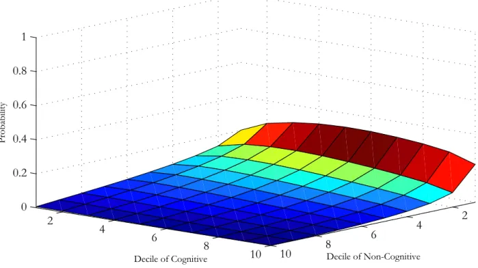
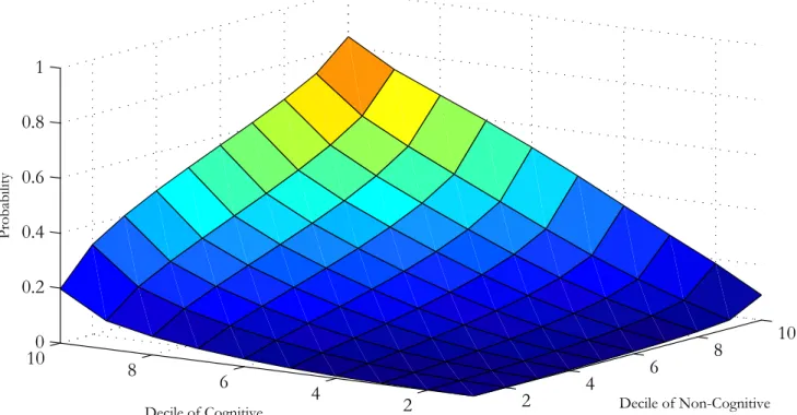
Wdeoh 7= Hvwlpdwhv ri Ydulrxv Uhwxuqv wr Rqh \hdu ri Froohjh

Idplo| Edfnjurxqg lv H{foxvlrq Idplo| Edfnjurxqg qrw H{foxvlrq f=f. ? S ? f=bH f=f. ? S ? f=bH

Dyhudjh Wuhdwphqw Hhfw 315457 31496;

+31397;, +313<49,

^31339<>315974` ^03133:7>315<88`

Wuhdwphqw rq wkh Wuhdwhg 316535 3155:<

+314436, +3144:4,

^313378>3173<7` ^0313369>316;53`

Wuhdwphqw rq wkh Xqwuhdwhg 314375 313;<:

+313;35, +3145;8,

^031335:>315855` ^0314733>316357`

Srolf| Uhohydqw Wuhdwphqw 3157;< 314<38

Hhfw +'833 Wxlwlrq Vxevlg|, +313;87, +314984,

^313357>316853` ^031436:>316935`

Ruglqdu| Ohdvw Vtxduhv 313:;; 313:<9

+3133<4, +313447,

^313987>313<88` ^313947>313<;6`

Lqvwuxphqwdo Yduldeohv 31497< 314863

+3136;<, +313:8;,

^313;;;>315499` ^313369>3157:<`

Qrwhv= Errwvwudsshg 80<8( vwdqgdug huuruv +lq sduhqwkhvlv, dqg frqghqfh lqwhuydov +lq eudfnhwv, duh suhvhqwhg ehorz wkh fruuhvsrqglqj frh!flhqwv +583 uhsolfdwlrqv,1

Vrxufh= Fduqhlur/ Khfnpdq dqg Y|wodflo +5338,1

Wdeoh 8= Lqvwuxphqwdo Yduldeohv Hvwlpdwhv

QOV\ 0 KV Judgxdwhv dqg Irxu0\hdu Froohjh Judgxdwhv Pdohv dw Djh 63^W

Lqvwuxphqwv Vwdqgdug LY LY0PWH +Frpprq Vxssruw,⁼

Ixoo Vdpsoh^_ Frpprq Vxssruw^h Sdudphwulf Sro|qrpldo Qrqsdudphwulf

Qxpehu ri Vleolqjv dw 47 31<;6 41455 316<3 31967 31967

+31845, +318<4, +31454, +31496, +31493,

Idplo| lqfrph lq 4<:< +wkrxvdqgv, 4199: 41;36 31749 318<3 31945

+31765, +31963, +31454, +31476, +3147:,

Orfdo Zdjh ri KV Judgxdwhv dw Frxqw| <71933 741733 3173: 318<4 3194;

Ohyho dw djh 4: +4:461633, +6671333, +31474, +3159<, +314<3,

Wzr \hdu Froo1 Judg*v orfdo zdjh dw djh 4: 8133; 816<7 31759 31933 31955

+713::, +71<74, +31468, +31549, +314;;,

Irxu \hdu Froo1 Judg*v orfdo zdjh dw djh 4: 51:75 6147< 3175; 31947 3195<

+413<6, +4186:, +31458, +314;:, +31495,

Orfdo Xqhps1 Udwh ri KV Judgxdwhv dw 319:8 31945 31536 31856 31859

Frxqw| Ohyho dw djh 4: +31937, +319:8, +31775, +661984, +4816::,

Wzr \hdu Froo1 Judg*v orfdo xqhpsor|phqw 31543 314;: 31696 318;3 318;;

udwh dw djh 4: +318:<, +31:5:, +31593, +41;57, +41<5:,

Irxu \hdu Froo1 Judg*v orfdo xqhpsor|phqw 61798 717;3 31738 31887 318;;

udwh dw djh 4: +4617:9, +4418;9, +31477, +315<7, +31553,

Glvwdqfh wr d wzr |hdu froohjh 6169< 71936 31749 31939 31954

+61556, +915;5, +3146<, +314;9, +31498,

Glvwdqfh wr d irxu |hdu froohjh 71;43 :1773 31748 3195< 31967

+814;3, +451483, +31453, +314:3, +31494,

Wzr |hdu froohjh wxlwlrq 05196: 041;:3 3174: 31:<; 319::

+61654, +514:5, +31:9:, +;19<3, +81<64,

Qrwhv wr Wdeoh 8

Zh h{foxghg wkh ryhuvdpsoh ri srru zklwhv dqg wkh plolwdu| vdpsoh1

|Wkh LY hvwlpdwhv dqg wkh vwdqgdug ghyldwlrqv +lq sduhqwkhvhv, duh frpsxwhg dsso|lqj wkh wudgl0 wlrqdo irupxodh wr wkh ixoo vdpsoh1 Wkh qxpehu ri revhuydwlrqv lq rxu vdpsoh lv <;51

}Wkh LY hvwlpdwhv dqg wkh vwdqgdug ghyldwlrqv +lq sduhqwkhvhv, duh frpsxwhg dsso|lqj wkh wudgl0 wlrqdo irupxodh wr wkh frpprq vxssruw vdpsoh1 Wklv vdpsoh frqwdlqv rqo| revhuydwlrqv iru zklfk wkh hvwlpdwhg surshqvlw| vfruh ehorqjv wr wkh frpprq vxssruw ri wkh surshqvlw| vfruh ehwzhhq wkh frqwuro +KV judgxdwhv, dqg wuhdwphqw jurxs +7 |hdu froohjh judgxdwhv, +<45 revhuydwlrqv,1

{Lq wkh uvw froxpq wkh LY hvwlpdwhv duh frpsxwhg e| wdnlqj wkh zhljkwhg vxp ri wkh PWH hv0 wlpdwhg xvlqj wkh sdudphwulf dssurdfk1 Lq wkh vhfrqg froxpq wkh LY hvwlpdwhv duh frpsxwhg e|

wdnlqj wkh zhljkwhg vxp ri wkh PWH hvwlpdwhg xvlqj d sro|qrpldo ri ghjuhh 7 wr dssur{lpdwh H+\mS,1 Wkh LY hvwlpdwhv lq wkh odvw froxpq duh frpsxwhg e| wdnlqj wkh zhljkwhg vxp ri wkh PWH hvwlpdwhg xvlqj wkh qrqsdudphwulf dssurdfk1 Wkh surshqvlw| vfruh +Sure+G @ 4m] @ },, lv frpsxwhg xvlqj wkh lqvwuxphqwv suhvhqwhg lq wkh wdeoh dv zhoo dv wzr gxpp| yduldeohv dv frqwurov iru wkh sodfh ri uhvlghqfh dw djh 47 +vrxwk dqg xuedq,/ dqg d vhw ri gxpp| yduldeohv frqwuroolqj iru wkh |hdu ri eluwk +4<8;04<96,1 Wkh vwdqgdug ghyldwlrqv +lq sduhqwkhvhv, duh rewdlqhg xvlqj errwvwudsslqj +433 gudzv,1

Vrxufh= Khfnpdq/ Xu}xd dqg Y|wodflo +5337,

Wdeoh 9= Wuhdwphqw Sdudphwhu Hvwlpdwhv

QOV\ 0 KV Judgxdwhv dqg Irxu0\hdu Froohjh Judgxdwhv Pdohv dw Djh 63^W

Wuhdwphqw Sdudphwhu^_ Sdudphwulf^h Sro|qrpldo^h Qrqsdudphwulf⁼

Wuhdwphqw rq wkh Wuhdwhg 31695 31:8; 319<9

+31456, +31534, +314;4,

Wuhdwphqw rq wkh Xqwuhdwhg 3183< 319;: 31985

+3147<, +31475, +3149:,

Dyhudjh Wuhdwphqw Hhfw 31788 31:46 3199;

+3145:, +31486, +31484,

ODWH Ef=S2> f=H 317;6 318< 3198<

+3146;, +314;8, +314<5, ODWH Ef=.b> f=DD 31888 4137 31:<5 +314:8, +3159<, +31578, ODWH Ef=eD> f=2 31745 3148: 316;6 +31453, +314;7, +3148<,

Qrwhv wr Wdeoh 9

WZh h{foxghg wkh ryhuvdpsoh ri srru zklwhv dqg wkh plolwdu| vdpsoh1

_Wkh wuhdwphqw sdudphwhuv duh hvwlpdwhg e| wdnlqj wkh zhljkwhg vxp ri wkh PWH hvwlpdwhg xvlqj d sro|qrpldo ri ghjuhh 7 wr dssur{lpdwh HE\ mS1

hWkh wuhdwphqw sdudphwhuv zhuh hvwlpdwhg e| wdnlqj wkh zhljkwhg vxp ri wkh PWH hvwlpdwhg xvlqj wkh sdudphwulf dssurdfk1

=Wkh wuhdwphqw sdudphwhuv zhuh hvwlpdwhg e| wdnlqj wkh zhljkwhg vxp ri wkh PWH hvwlpdwhg xvlqj wkh qrqsdudphwulf dssurdfk1 Wkh vwdqgdug ghyldwlrqv +lq sduhqwkhvhv, duh frpsxwhg xvlqj errwvwudsslqj +433 gudzv,1 Vrxufh= Khfnpdq/ Xu}xd dqg Y|wodflo +5337,

î.50.511.52

MTE

0 .1 .2 .3 .4 .5 .6 .7 .8 .9 1

v

MTE CI(0.025,0.975)

Source: Heckman, Urzua and Vytlacil (2004).

The dependent variable in the outcome equation is hourly earnings at age 30. The controls in the outcome equations are tenure, tenure squared, experience,

Sample of HS Graduates and Four Year College Graduates î Males at age 30 î Nonparametric

Figure 7. MTE with Confidence Interval

0.005.01.015.02 Prop. Score’s Weights

0.005.01.015.02

Four year college tuition’s Weights

0 .1 .2 .3 .4 .5 .6 .7 .8 .9 1

v

Four year college tuition Propensity Score

Source: Heckman, Urzua and Vytlacil (2004).

The dependent variable in the outcome equation is hourly earnings at age 30. The controls in the outcome equations are tenure, tenure squared, experience,

corrected AFQT, black (dummy), hispanic (dummy), marital status, and years of schooling. Let D=0 denote dropout status, and D=1 denote GED status. The model for D (choice model) includes as controls the corrected AFQT, number of siblings, father’s education, mother’s education, family income at age 17, local GED costs, broken home at age 14, average local wage at age 17 for dropouts and high school graduates, local unemployment rate at age 17 for dropouts and high school graduates, the dummy variables black and hispanics, and a set of dummy variables controlling for the year of birth. The choice model is estimated using a probit model. In computing the MTE, the bandwidth in the first step is selected using the leaveîoneîout crossîvalidation method. In the

Propensity Score vs Four year college tuition as the Instrument

NLSY î Sample of HS Graduates and Four Year College Graduates î Males at age 30

Figure 8a. IV Weights

0.005.01.015.02 Prop. Score’s Weights

î.04î.020.02.04

Two year college tuition’s Weights

0 .1 .2 .3 .4 .5 .6 .7 .8 .9 1

v

Two year college tuition Propensity Score

Source: Heckman, Urzua and Vytlacil (2004).

The dependent variable in the outcome equation is hourly earnings at age 30. The controls in the outcome equations are tenure, tenure squared, experience,

Propensity Score vs Two year college tuition as the Instrument

NLSY î Sample of HS Graduates and Four Year College Graduates î Males at age 30

Figure 8b. IV Weights

Ex Ante and Ex Post Returns: Distinguishing Heterogeneity from Uncertainty

• Panel data earnings studies Lillard and Willis (1978) and MaCurdy (1982) estimate earnings equations:

\_l>w = [_l>w + V_l + X_l>w (8)

• \_l>w> [_l>w> V_l> X_l>w denote (for person l at time w) the real- ized earnings, observable characteristics.

X_l>w = !_l + _l>w (9)

• Alternative specification

X_l>w = _lw + %_l>w

• _l is a vector of skills (e.g., ability, initial human capital, motivation, and the like).

• _w is a vector of skill prices.

• %_l>w are mutually independent mean zero shocks indepen-

dent of _l.

A Generalized Roy Model

• V_l denote dierent schooling levels.

V_l = 0 denotes choice of the high school sector for person l.

V_l = 1 denotes choice of the college sector.

• Denote by F_l the direct cost of choosing sector 1.

• \_1>l is the ex post present value of earnings in the college sector,

\_1>l =

XW w=0

\_1>l>w (1 + u)^w >

• \_0>l is the ex post present value of earnings in the high

school sector at age zero,

\_0>l =

XW w=0

\_0>l>w (1 + u)^w =

• u is the one-period risk-free interest rate.

• \_1>l and \_0>l can be constructed from time series:

(\0>l>0> = = = > \0>l>W).

• Practical problem, we only observe one or the other of these streams.

• \_1>l> \_0>l> and F_l are ex post realizations of returns and costs.

• Il>0 denote the information set of agent l at the time the

schooling choice is made, V_l =

½ 1> if H (\_1>l \_0>l F_l | Il>0) 0

0> otherwise. (10)

Identifying Information Sets in a Linear Equation Example

Write discounted lifetime earnings of person l as

\_l = + _lV_l + X_l (11) _l = _l + _l

_l is a component known to the agent _l is revealed after the choice is made.

V_l = (_l> ]_l> _l)

V_l = ₀ + _1l + _2l + ₃]_l + _l (12) ] and the proxy costs and with X

Suppose that agents do not know _l=

• Using Becker (1967) — Rosen (1977) — Card (2001) model must be extended to account for uncertainty, under ra- tional expectations

V_l = ¯ u_l n =

• Ex Post earnings observed after schooling are

\_l = ¯ + ¯V_l + {(_l ¯) + (_l ¯) V_l} =

• Suppose that we observe u_l, u_l independent of (X_l> _l) =

Observe that if agent knows _l and acts on it, we can construct it

V_l = _l u_l n so

_l = u_l + nV_l=

• If agents do not know _l and there is no selection bias (FRY (V_l> X_l) = 0)

FRY (\> V) = ¯Y du (V)

because (_l ¯) is independent of V_l and (¯> ¯) because V_l BB [(_l ¯) > (_l ¯) V_l] =

• If, on the other hand, agents know _l> OLS breaks down.

• Instrument with u_l.

• In this case,

FRY (\_l> V) = ¯Y du (V) + FRY| (V>{z( ¯) V}) =

We observe V> can identify ¯ and can construct ( ¯) for each V.

• The extra piece of the variance is due to information by agent.

• Method breaks down when there is selection bias FRY (X_l> V_l) 6= 0.

• Need a more general method (Cunha, Heckman and Navarro 2005a,b,c,d and at this World Congress).

Identifying Information Sets

• Cunha, Heckman and Navarro (2005a,b,c,d)

• Suppose, contrary to what is possible, that the analyst observes \_0>l, \_1>l, and F_l.

• Such information would come from an ideal data set in which we could observe two dierent lifetime earnings streams for the same person in high school and in college as well as the costs they pay for attending college.

• From such information, we could construct \_1>l\_0>lF_l.

• Could also construct H (\_1>l \_0>l F_l | Il>0).

• Under the correct model of expectations, we could form the residual

Y_Il>0 = (\_1>l \_0>l F_l) H (\_1>l \_0>l F_l | Il>0) >

for the ex ante college choice decision.

• A test for correct specification of candidate information set Iel>0 is a test of whether V_l depends on Y_Ihl>0,

Y_Ihl>0 = (\_1>l \_0>l F_l) H ³

\_1>l \_0>l F_l | Iel>0

´

=

• Information set is correct if V_l BB Y_Ihl>0 | Iel>0.

• In terms of the simple linear schooling model of equations (11) and (12), condition says that _l should not enter the schooling choice equation (₂ = 0)=

• A test of misspecification of Iel>0 is a test of whether the coe!cient of Y_Ihl>0 is statistically significantly dierent from zero in the schooling choice equation.

• Iel>0 is the correct information set if Y_Ihl>0 does not help to predict schooling.

• Extensions by Carneiro, Hansen and Heckman and Cunha, Heckman and Navarro (this World Congress) and Navarro account for imperfect credit markets (of varying types), risk aversion and add consumption data.

Preferences, Market Structures and Rates of Return

• Open question, not yet fully resolved in the literature:

• How far one can go in nonparametrically jointly identify- ing preferences, market structures and information sets?

• Cunha, Heckman and Navarro (2005c) add consumption data to the schooling choice and earnings data to se- cure identification of risk preference parameters (within a parametric family) and information sets, and to test among alternative models for market environments.

Evidence on Uncertainty and Heterogeneity of Returns

• Large psychic costs components.

• is big and is not negligible as has been assumed in early literature.

• Ability is an important determinant of these costs.

• Costs could be expectational errors; not credit constraints.

• This evidence of substantial psychic costs is robust across many specifications of credit markets.

• Uncertainty important quantitatively.

• Convention in the literature that equates variability with uncertainty is incorrect.

• Estimated risk aversion coe!cient 2.15.