After a comparison between 𝐶𝑀𝛼 of the rigid, the linear deformed and the non-linear deformed wing took place. The calculation of the dynamic stability derivatives is more sophisticated and different approaches were investigated by researchers. Due to the limited time schedule for the work, an assessment of the dynamic stability derivatives was out of scope.
The main objective of this work is to investigate the characteristics of a preliminarily designed high aspect ratio airfoil. To get an idea of the flight stability, a brief introduction to stability derivatives is given. Parameters affecting the divergence speed are the torsional stiffness of the wing and the distance.
Therefore, it is extremely important to know the behavior of the aircraft for the quality of the flight.
![Figure 2-1: Aeroelastic Triangle of Forces with a selection of phenomena, adapted from [22]](https://thumb-eu.123doks.com/thumbv2/123dok_br/19768225.0/17.892.107.786.441.883/figure-aeroelastic-triangle-forces-selection-phenomena-adapted-22.webp)
Multidisciplinary Design Optimization (MDO) Tool
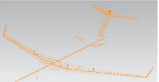
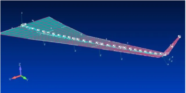
In this chapter, an overview of the used programs as well as the corresponding theory for solution is given. In the first part of the flight characteristic investigation, the flapping speed was estimated to ensure that the wing could be operated in the desired speed range. For this, the programs used were: a multidisciplinary design optimization tool (MDOGUI) for the aeroelastic deformation of the wing; Nastran for the fluttering determination; and MATLAB as a tool.
By integrating the integrals of formula (5-3) for each surface panel, the so-called aerodynamic influence coefficients can be obtained and the problem can be solved. Differentiation yields the tangential velocity for each panel and Bernoulli's potential flow equation allows the pressure to be calculated. To obtain more information about the implementation of the aerodynamic model, reference is made to the associated literature [38, 39].
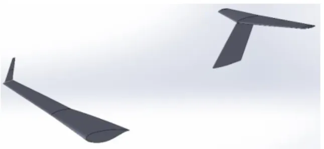
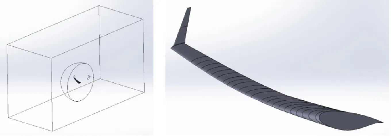
The wing structure is modeled as a flexible beam as it captures the most important features. The stress field {𝜎}, as in the case of an isotropic and elastic material, can be written with the elasticity matrix [𝐷]. More detailed information can be gathered from the reference literature for the tool [38, 39] and the method [41].
It is monolithic, as the solution progresses with the convergence between the structural and aerodynamic model. It is also loosely coupled, as the structural and aerodynamic models are computed independently and merged with the FSI algorithm [38]. Therefore, the loads from the aerodynamic structure are transmitted to the structure, and the displacements are transmitted vice versa.
MSC Nastran
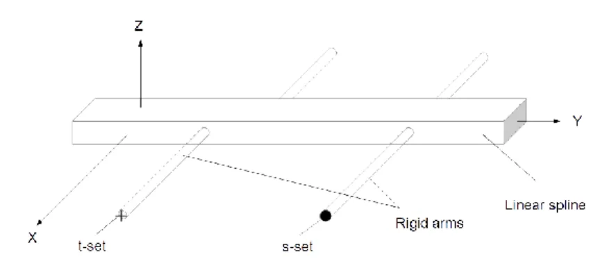
To calculate the aeroelastic behavior, a coupling between the aerodynamic and the structural model is required. Their edges are aligned with the flow direction of the free stream and the fold and hinge lines are on their boundaries. The independence of the structural and aerodynamic grids allows each of them to be optimally adapted to the conditions and the chosen theory.
In Nastran, the aerodynamic degrees of freedom are dependent, while the structural are independent. In short, two transformations are needed, one that interpolates the structural to the aerodynamic deflections and another for the relationship between the aerodynamic forces and the structurally equivalent forces occurring at the structural grid points. The structural and aerodynamic grids must interact and are connected by interpolation, which is done by so-called splines.
With this method, the deformation of the two models, structural and aerodynamic, is tried to match ("structurally equivalent"). An aeroelastic dynamic problem can be formulated as: the DOFs of the systems with its derivatives and the {𝐹} load vector. The latter is the sum of the force of gravity [𝑀]{𝑔}, the aerodynamic stiffness matrix [𝐴𝐾] and the aerodynamic damping matrix [𝐴𝐶]:.
The necessary transformations complement the structural model using splines and a model reduction to achieve the general form. True roots indicate a convergence or divergence, as in the case of the roll subsidence (rigid body) or a structural (torsion) [42]. Still, most eigenvalues will be conjugate complex pairs and the oscillatory solutions of equation (5-25) require iterative computation in such a way that equation (5-27) is satisfied together with equation (5-25).
MATLAB
The roll immersion root or static structural divergence roots require no iteration and are found by setting 𝑘 = 0. The oscillating rigid body roots and oscillating roots are found by an algorithm detailed in [42]. However, the goal is to determine stability at a given speed independent of stability at lower or higher speeds.
An advantage of using the p-k method is the production of results directly for a given set of speeds instead of necessary iterations to calculate the reduced frequency of flutter. The estimated damping in the algorithm is also more realistic than the purely mathematical expression of Equation (5-29).
SolidWorks
ANSYS
The value of the moment was 1𝑥106𝑁𝑚 to get a good comparable displacement as well as for the single point loads. For the applied loads, one can recognize the good agreement for the deflections in the z direction, which will be af. For the dynamic behavior, on Figure 7-3: Comparison of linear and nonlinear displacement to increase the angle of attack.
Figure 7-4 shows the trend for natural frequencies versus tip displacement for linear and nonlinear wings. In the following, the calculation of the flutter speed for the wing will be described and the results obtained will be discussed. An example result for an angle of attack of 10° for a linearly deformed wing is presented in Figure 7-6 and Figure 7-7.
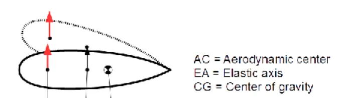
For the spin mode, the wing twist increases as the angle of attack increases, which appears to have an inverse effect on the flutter speed. While the slope of the flutter speed for the rigid wing is negative, the flexible wings have a behavior in the opposite direction. For an arbitrary cross section of the wing, about 50% of the chord length can be assumed for the width of the wing box and the entire height of the section for the box height.
Flutter borders for plane mode and rotate mode are drawn separately for better overview. The trend of the corrugation limit is the same for the reduced thickness, as expected. In Figure 8-2, the trend for the flutter velocity is shown and it can be seen that for the in-plane mode the difference between the linear and non-linear arm is increasing with decreasing thickness.
Contrary to this trend, the difference of the speeds for the torsional mode remains almost constant and the non-linear deformed wing even has its second flutter speed a little earlier. With a resulting mass reduction of 7.3%, the flutter limit decreases between 3% and 6% for the calculated angles of attack for the linear and non-linear deformed wing.

Mesh convergence study
At the beginning, a mesh convergence study was performed to find a good balance between computational cost and accuracy. This was followed by steady flow solutions for the rigid and deformed wing for various angles of attack. The calculated y+, a dimensionless wall distance parameter, within Ansys and with those boundary conditions is about 200 for the wing, which is sufficient for the used turbulence model (SST), since ANSYS has an internal correction factor (according to the help documentation).
The shear stress transport turbulence model is a mixture of the 𝑘 − − and − 𝜔 models, which automatically switch in the CFX environment in the wake region from 𝑘 − 𝜔 to 𝑘 − 𝜖. The Reynolds number for the present case is about 30 million, with a reference length of 2.5 m and a free stream velocity of 200 m/s at sea level (corresponding to 0.59 Ma). The calculation range of interest was between -2° and 10° angle of attack, for which wing deformation was previously calculated with the MDO tool.
𝐶𝑚𝛼 Due to the deformation, the lift curve is flatter for the deformed wing, while the nonlinear deformed wing still has a higher and steeper lift curve since its displacement is slightly lower.
Results for static stability derivatives
The evaluation of the lift, drag and moment coefficients was done for a range from -2° angle of attack to 10° angle of attack. It is clearly noticeable that the lift slope and moment coefficient are lower for the deformed wings. As mentioned earlier, due to the distance between the calculation points, a trend can be noticed, but possible deviations between the individual points could not be noticed.
This thesis aimed to investigate the influence of geometric nonlinearities of structural deflections on the flight performance of a preliminarily designed wing. The result for this specific wing was a low difference between displacements of the two deformed wings. The results show an almost reduced linear trend, where the geometric reduction of 10% leads to a reduction of flutter speed of approximately 5% for the different angles of attack.
For stability behavior, only a longitudinal static stability (𝐶𝑀𝛼) derivative could be investigated in the scope of the work. The slope of the deformed wings is thereby lower than for the idealized rigid wing. First, further parametric studies could be performed and the magnitude of the influence on the stability derivatives could be investigated.
Here, a determination of the dynamic stability behavior (derivatives) would be interesting, since with the deformations a more clear response could be expected due to the high aspect ratio. Proceedings of the Institution of Mechanical Engineers, Part G: Journal of Aerospace Engineering, Vol 231, Issue 10, pp Hassig, "An Approximate True Damping Solution of the Flutter Equation by Determinant Iteration," Journal of Aircraft, Vol 8, No 11 , p.
Appendix A - 2: Linear deformed wing flap plots of the changing angles of attack at sea level and the deformation data from 200 m/s. Appendix A - 3: Nonlinear deformed wing flap plots of the changing angles of attack at sea level and the deformation data from 200 m/s.
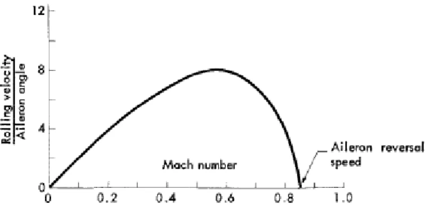
![Figure 2-3: Aileron effectiveness dependent on speed, from [23]](https://thumb-eu.123doks.com/thumbv2/123dok_br/19768225.0/18.892.122.768.992.1131/figure-2-3-aileron-effectiveness-dependent-speed-23.webp)