The aim of the thesis is to create a model for electricity load forecasting using machine learning and activity models. By using holiday information and applied statistical methods, datasets were enriched with additional information that was used as input to the machine learning model. Various machine learning models, namely: random regression trees, gradient boosting regression, and neural networks with LSTM cells, have been implemented and tested to predict electricity consumption one hour ahead to target values one day ahead.
A implementação de modelos de aprendizagem automática pode incluir diversas aplicações de negócio que otimizam os custos de utilização da rede, tais como a implementação de modelos de resposta à procura ou controladores inteligentes fora da rede. O objetivo desta tese é criar um modelo para prever o consumo de eletricidade usando algoritmos de aprendizado de máquina e análise de padrões de atividade. Desta forma, os dados do estudo de caso foram enriquecidos com essas informações para aplicação de métodos de aprendizado de máquina.
Diferentes métodos de aprendizagem automática foram desenvolvidos e testados, nomeadamente: árvores de regressão aleatória, regressão gradiente boost e redes neurais com LSTM, para prever o consumo de eletricidade na próxima hora e no dia seguinte.
Introduction
- Problem definition
- Research goal
- Research questions
- Structure of the document
The research goal of the thesis is to develop a model that will accurately predict electricity consumption with different time horizons of the future. Electricity forecasting – determination of model performance measured by mean absolute error, mean square error and coefficient of determination; Response Time – Model latency determines the model's ability to operate on real-time data.
What are the strategies and methods that can improve the predictive ability of the model. The selected algorithms are described in detail from the perspective of the mechanisms and logic behind their formulation. Based on the prediction results, several performance metrics were calculated with the aim of determining the applicability of the algorithms to real-time data.
In the business application section of the solutions section, possible business applications for the proposed methods are presented.
Literature review
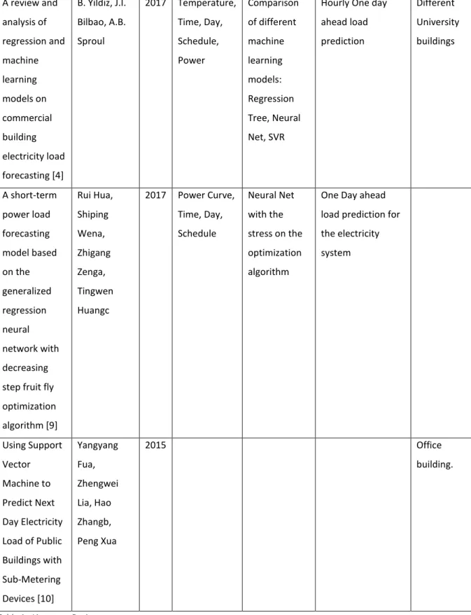
In [1] the authors focus on developing a model that will predict electricity consumption for the next 24 hours at the individual household level. The authors achieved mean absolute percentage errors (MAPE) equal to 41.7% and 23.64% in the case of the best performing model for two different datasets. The authors tested several machine learning techniques for prediction: regression trees, neural networks, and support vector regressions.
In [7], the authors developed a demand response model for large commercial buildings using regression stress. The authors integrated several machine learning algorithms into one system, which improved the overall prediction ability of the system. Moreover, the authors showed that the use of real-time machine learning-based algorithms combined with elastic electricity tariff systems.
In [5], the authors developed a machine learning model for the national power system for 24-hour electricity demand forecasting.
Methodology
Exploratory data analysis
- Description of the analyzed case studies
- Data transformation procedure
Information about meteorological data: temperature, pressure and wind speed has been added for the Restaurant dataset. The result of the following procedure is a vector of 36 features that was used as input into the machine learning models. Statistical data such as mean, standard deviation, maximum and minimum value were calculated on the data set.
Machine learning algorithms
- Gradient Boosting Regression Trees
- Random Forest Regression Trees
- Long short-term memory (LSTM) recurrent neural network
Gradient descent procedure is used to minimize loss when adding trees – after calculating error or loss in the function, coefficients in a regression equation are updated to minimize that error. After updating coefficients for each tree, all outputs are combined in an attempt to improve the final output of the model. Random Forest is a supervised learning algorithm from the group of decision trees, which, based on small subsets of data, creates a whole group of trees by merging them to obtain an accurate final prediction.
The disadvantage of the algorithm is that some individual trees can be trained on data that is very specific and does not provide a good perspective on the overall structure of the data set. A single decision tree is trained on the random sample using the most optimal partition to predict the target value. Given the test data, each tree comes up with the prediction, and the prediction that was predicted by the most individual trees is taken as a model.
In other words, the LSTM cell can take advantage of the information that occurred in the past and is not a current input to the model as opposed to the regular neural network that only takes current input as input information. LSTM cells have a chain structure, meaning that the output weights from one cell are input to the next along with new input data. The defining element of the LSTM cell is a cell state, which is represented by the horizontal line at the top of the diagram shown in Figure 1.
The LSTM adds an information or removes an information to the cell state using the activation functions which can be either sigmoid or tanh one. Output weights from the previous cell (represented by t-1 in the Figure 1) together with the cell state and new input are delivered as input parameters to the cell (represented by t in the Figure 1). Based on the new information and forgetting factor which are both controlled by different activation functions, the cell state is updated.
Cell state and weights are sent as input to the next cell (represented by t+1 in Figure 1). A series of cells form an LSTM network that can either output the prediction value at each step, as shown in Figure 1 (many-to-many network), or output a single value at the end of the network (many-to-one network).
Metrics used in the validation of the machine learning algorithm
- Mean squared error (MSE)
- Mean absolute error (MAE)
- Coefficient of determination (R 2 )
- Pearson correlation coefficient
Results & Discussion
Exploratory analysis
- Blood analysis clinic A dataset
- Blood analysis clinic B Clinics dataset
- Restaurant dataset
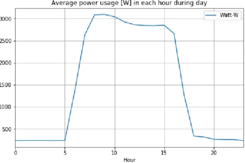
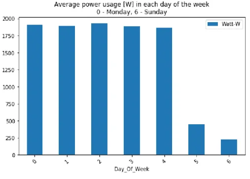
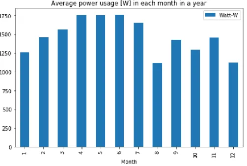
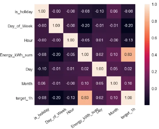
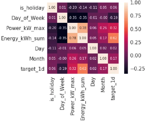
Two periods of electricity consumption can be distinguished: at night, when the average consumption is equal to 200 W (probably taking into account the basic consumption of the building) and during the day, when the average consumption is equal to 2700 W. The lowest consumption is on average on Sunday. , while the highest is on Wednesday. The highest average energy consumption is in June and the lowest in August (holidays).
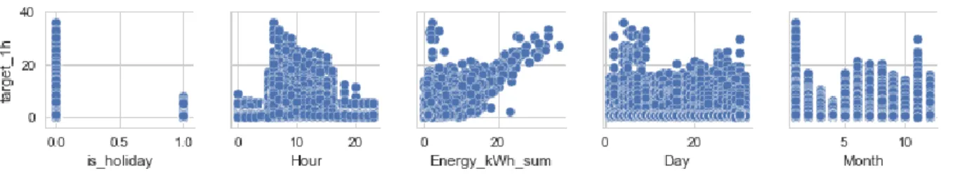
The target value shown on the vertical axis is a value of electricity consumption for the forecast 1 hour ahead. As it can be observed that there is a clear correlation between electricity consumption and a target value which has a Pearson coefficient equal to 0.83. This correlation means that as electricity consumption increases, so does the value of the electricity forecast.
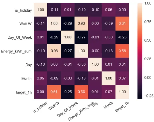
Three periods of electricity consumption can be distinguished: night when the average consumption is equal to 1000W (probably this is responsible for the base consumption of the building), morning high electricity consumption from 6am to 11am and afternoon medium level electricity consumption from 11am to 5pm. There is a big difference between weekdays and every day of a weekend in average power consumption. The lowest power consumption occurs on Sunday, while the highest occurs on Monday.
It can be seen that there is a clear correlation between electricity consumption and the target value, which has a Pearson coefficient equal to 0.61. We can distinguish two periods of electricity consumption: at night, when the average consumption is equal to 5000 W (probably taking into account the basic consumption of the building) and during the day with a clear peak consumption at 1 pm, which amounts to 16,000 W. The lowest energy consumption takes place on Sunday, the highest and on Thursday.
From the figure, it can be concluded that cooling season occurs from May to August when average power is greater than 8000 W. There is a clear difference in the night and day power consumption in all three analyzed datasets. There is a clear difference in power consumption between working days (from Monday to Friday) and weekend days (Saturday and Sunday).
The presence of a seasonal cooling that occurs in July and August is a conclusion that can be drawn from the monthly power consumption aggregation.
Random forest regression
- Blood analysis clinic A Dataset
- Blood analysis clinic B Dataset
- Restaurant Dataset
Based on the input variables described in the Data transformation procedure section, the following results were obtained.
Gradient boosting regression
- Blood analysis clinic A Dataset
- Blood analysis clinic B Dataset
- Restaurant Dataset
RNN with LSTM cell
- Blood analysis clinic B Dataset
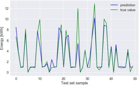
Due to the long calculation time and limited resources of computing power, only the data set of the Blood Analysis Clinic B was analyzed. From the figure, we can conclude that at the end of the training process, the model reaches the plateau phase, which means that the training limit has been reached. To improve performance, you can increase the number of epochs or increase the network size (this is not possible in this project due to computing power limitations).
We can see that the predicted values cover the actual values, which is also the goal of the predictive model. It should be emphasized that neural networks perform very well when the dataset size is large, so that the training process can be performed accurately and the loss function can be optimized on different data.

Different resolution of predicted values (one hour ahead, one day ahead)
- Dataset description
- Random Forest Regression – Results
- Gradient Boosting Regression - Results
One can conclude that due to the small size of the data set, the overfitting problem is very evident. For that reason, it is difficult to tune the performance of the model on the validation and test set.
Discussion
- What are the cyclic patterns that can be observed form the data produced by different types of
- What are the strategies and methods that can improve the forecasting ability of the model?
- Does the same model perform equally on two different datasets?
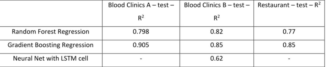
Results provided in Table 22 show that the same model performs differently on two different data sets. With the high variance in the input data, the training part is crucial to achieve appropriate results and predictions on the data set. For that reason, it can be stated that to achieve good prediction ability, the training period cannot be omitted.
However, in each model analyzed, the value of the amount of past electricity consumption had the greatest impact on predictive ability.
Business application of the solution
How the solution can be implemented
What are the possible markets that could benefit from those algorithms
Potential benefits for the user
Conclusions

![Figure 1 - LSTM neural net schema. Source: [17]](https://thumb-eu.123doks.com/thumbv2/123dok_br/19779579.0/19.892.121.768.223.472/figure-1-lstm-neural-net-schema-source-17.webp)