A renormalization of the gap was estimated for both the undoped and hole-doped system. Units: me) 35 4.1 Renormalization of the half-band gaps for the spin-split valence band, forεr= 1.
The discovery of graphene and the rise of 2D-materials
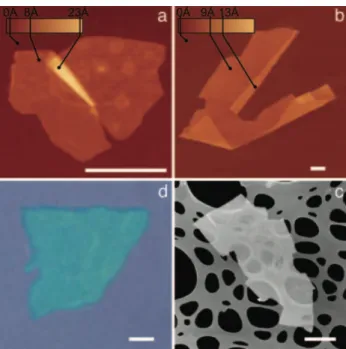
Despite the reduced thickness, the layers of graphene managed to produce a small interference which could be observed against the bare surface with an optical microscope [2, 9] (Fig. 1.1). Although graphene attracted the limelight among the brand new class of 2D materials, certainly due to both its vast new landscape of physics as well as its potential for device applications [20], it has been in extremely good company since as early as BN , Bi2Sr2CaCu2Ox, NbSe2 and MoS2.
The superlatives and the shortcomings of graphene
Band gap An early renormalization group analysis of electroelectron interactions showed no band gap in single-layer graphene, a result that has been experimentally verified [29]. One of the most effective ways to increase DOS at the Dirac point is to create vacancies in the carbon lattice, inducing zero energy states [40, 41].
A companion family: Group-VI transition metal dichalcogenides
Due to the weak screen of Coulomb interactions in 2D materials, strong excitonic effects become apparent. In addition, due to the large spin splitting of the valence band at the K point, two excitonic features are found in the photoabsorption spectrum [25].
Outline
Discrete symmetries of the Hamiltonian and Group Theory analysis
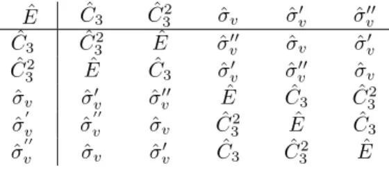
The calculation of the TB Hamiltonian matrix will be based on the basic relation for the one-electron Hamiltonian. The remaining operations can be derived from the subset multiplication table, as shown in Table 2.1.
Representations and computation of hopping matrices
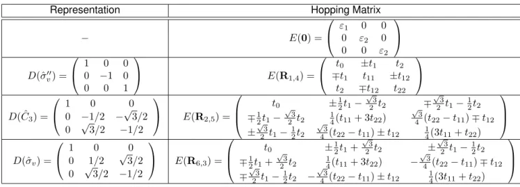
A summary of the representations of the relevant operations and the resulting jump matrices can be found in Table 2.2. Note that the Fourier transform of the creation and annihilation operators induces a Fourier transform from the Wannier states to the Bloch states of the orbitals, so the TB Hamiltonian is written in the basis{|ϕα(k)i}∀k,α given by.
Spinful tight-binding Hamiltonian
Basis states and tight-binding Hamiltonian with spin-orbit coupling
To evaluate the matrix elements of the SOC term, note that it can be written as (which implies tensor products). It is no surprise that the application of the operator produces states outside the Hilbert space under consideration.
Taylor expansion of the TB Hamiltonian
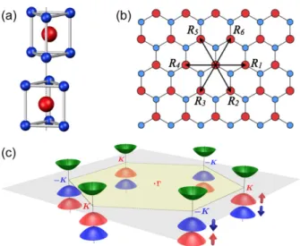
To understand why, notice the orbital composition of the valence and conduction bands near the K points. The inclusion of the valley index in the spin-splitting term is due to the fact that the +K and -K valleys are associated with time reversal.

Effective masses
Here the electron-hole symmetry is clear: in the first order, the masses of the valence and conduction bands are equal. Note that the spin splitting is substantial enough to make, in all cases except MoS2, the high cone of the valence band less massive than the conduction band.
Hall effects in inversion symmetry broken honeycomb lattices
- Berry connection and Berry curvature
- Hall conductivity
- Tight-binding description of electronic interactions
- Evaluation of the matrix elements of the interaction
Therefore, the Berry relation becomes Avµ(k) =τ3εµαkα. which is the Berry curvature in a vicinity of ± K-points:. To solve this, it is useful to go to the definition of the Berry curvature in terms of the first-order adiabatic evolution of quantum states of Sec. Therefore, the contour of the Berry curvature integral should go no further than half the magnitudes in the nearest valleys.
We are interested in studying electronic interactions in the low energy limit of the tight-binding model.
Gap renormalization
- Undoped system
- Hole-doped system
- Intra- and inter-orbital couplings, validity of the Hubbard model
- Path-integral formulation
This result can be obtained as a static low energy limit of the random phase approximation (RPA) [115]. This implies that the only DOS contributing to the screening are those from the high elevation cones from the two dissimilar valleys. In the next chapter we will show that higher doping regimes are most likely experimentally inaccessible, so we can safely create an energy-efficient approximation for the DOS by using a parabolic approximation of the spectrum at the valence edge. band.
We are now in a position to determine the renormalization of the gap due to hole doping.
Low-energy theory
Saddle-point solution
On the other hand, the configuration that minimizes the performance is expected to be the dominant contribution to the large partition function based on the path integral structure. The first is related to the position of the Fermi level, lowered by hole doping, and the subsequent shift of the spin-split cones. The second concerns the description of the energy spectrum of a low-energy system.
More precisely, we consider to be within the range of validity of the parabolic approximation for the valence band.
Action expansion
However, we will make use of the solution arrived at here, which corresponds to the saddle point solution of the action that applies to the normal phase. D{δφτσ}e−S0[{δφτσ, where Z0 is the grand partition function of the non-interactive system and the newφ field action S0reads. This ansatz is variational in the sense that the solution will be determined by virtue of minimizing the action: corresponding to the motivation of Eq. 5.8), the structure of the path integral Eq. 5.18) is such that the solutions that minimize the action constitute the dominant contribution to the grand-partition function.
Why is this approach necessary, considering that it is basically based on the same principle as the previous one. 5.12) suggests that the saddle point solution does not account for a minimum in the broken symmetry phase, so we must look a little more broadly at the action near the transition.

Anomalous Hall effect in the spin-valley-polarized phase
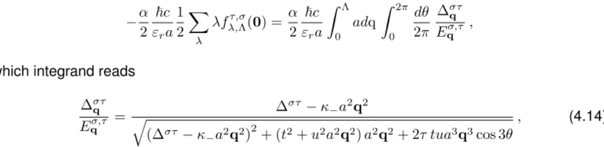
5.34, and assuming that the system is doped only slightly below the maximum of the high-lying cones, we can expand the square root to 1st order, which yields. The upper limit of this threshold is set in terms of the ionizing electric field magnitude for hydrogen. We previously determined the threshold values µA and µB for entry into the medium and high doping regime, respectively.
Within the validity of the parabolic approximation, the relationship between the hole surface densityρ and the Fermi level µ0 is given by.

Dependence on the Fermi level
Note that the 1st-order term vanishes identically, by virtue of charge conservation, Eq. 5.27) and (5.28) to decouple the variational parameters in quadratic terms, we can write the unphysical action as. Clearly, the critical value of the Hubbard coupling constant within the intermediate doping regime is again given by . Note that the conductivity is actually continuous with the conductivity in the low-doping regime, although the 1st derivative is not.
Finally, the shift of the Fermi level in the broken symmetry phase δµ∗ is given by.
We can now write the perturbation in terms of band states at point K. Therefore, the total Hamiltonian at point K in terms of band states is Indeed, we should expect that perturbation will mix subspace states with other states.
This means that the rate of change of the system parameters P(t) is negligible, P˙ →0.

Quantum adiabatic theorem
Moreover, a quantum system will initially remain in an eigenstate |n(P(0))i as an instantaneous eigenstate of the Hamiltonian H(P) under adiabatic evolution. Here, adiabatic is understood as in the thermodynamic definition: that the system evolves slowly enough so that the system can adapt to the new configuration at every moment. Despite this fact, since the rise of quantum mechanics and until the work by Berry [121], this phase has been neglected in the study of quantum dynamics, since its elimination amounts to a gauge transformation.
A correct choice of the calibration function can therefore eliminate γn(t), leaving only the dynamic phase, making it unobservable.
Berry phase and Berry curvature
Note that we did not refer to the specificity of the physical system when arguing this result. Indeed, the only condition is the periodicity of the parameter space and, therefore, of the Hamiltonian. Some important symmetries and conservation laws of Berry's curvature can be obtained directly from its definition.
To explore the deeper consequences of the Berry curvature on Bloch electron dynamics, we need to consider the perturbative effect of residual eigenstates on the evolution of the unperturbed eigenstate.
Bloch bands and Hall effects
- Brillouin zone as a parameter space
- Velocity under adiabatic evolution
- Bloch electrons in an electric field
- Grand-partition function of a non-interacting theory
- Green’s functions - bare propagator
- Matsubara frequency sums
Therefore, it is possible to take the Brillouin Zone as the parameter space of the HamiltonianH(q) with eigenbasis{|n(q)i}. As expected, the Fourier transform of the propagator of a time-homogeneous system is diagonal in frequency-space. The second term can be obtained simply by interchanging the fields in the first equality of the above equation, that is.
We begin by noting that the propagator has two parts, based on the time ordering operator.
Green’s functions - Perturbation Theory
Dyson’s equations, self-energy correction of the bare propagator
The process described above can indeed make relevant contributions to all orders of the perturbative expansion. Although we do not aim for a formal proof, we can present the following schematic argument: since the order of the perturbative expansion is represented by the sum of the diagrams resulting from each coherent combination of interaction diagrams of Figure 4.1 (in the main text), will each sequence contains a term corresponding to the then-fold multiplication of the diagram of Fig.
However, such an approach is analytically intractable, so it is a common approach to approximate it by the contribution of the first-order exchange process by virtue of the physically motivated argument presented above.
Conservation of crystal momentum from the Coulomb potential
Due to the thermodynamic relation Ω' F −µhN i, which is valid in the thermodynamic limit, we can write the following inequality for the free energy F,. AtT →0and within the parabolic approximation, similar to the main text, we have. We keep this discussion to the low doping regime described in the main text, in which case it reads as internal energy.
In the main text, we derived the effective action of the field φ from the H-S action equation. 5.7), which after creating the appropriate ansatz of Eqs.