Fast Associative Memory

INTRODUCTION

M OTIVATION

O BJECTIVES

S OLUTION

D ISSERTATION S TRUCTURE

OVERVIEW – RELATED WORK

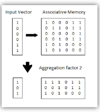
A SSOCIATIVE M EMORY

One aspect of the pattern present in the vector is represented by one component. In the hard threshold strategy, T is set to a minimum number of one component in each memory unit.

H OPFIELD N ETWORKS

L is the number of vector pairs that can be stored in this model before errors start to occur in the retrieval phase. In the above formula, D represents the number of class patterns to be stored in the network; n is the dimension of the class pattern vectors.

SDM – S PARSE D ISTRIBUTED M EMORY

As for the capacity of the Hopfield Networks model, it has been calculated to be approximately 0.15n, where n refers to the number of units (11). Another important property of high-dimensional space has to do with the distances between points.

BAM - B IDIRECTIONAL A SSOCIATIVE M EMORY

Another property that can be verified, and which is not shared by all associative memories, is that the SDM is not only tolerant of corruption in the address, but also tolerant of noise in the data (15). Regarding the capacity of the SDM model, James Keeler has shown that the binary Hopfield Network and the sparse distributed memory models have the same capacity per storage element (0.15n) (30).

A PPLICATIONS

Associative Memory for text documents
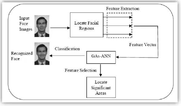
Associative Memory in face recognition
Associative Memory in gesture recognition and training
Associative Memory in voice recognition and training
Associative Memory in music classification

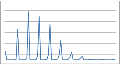
In each test, the size of the binary vectors in the associative memory is 1000 elements. As intended, the number of ones in memory will be higher than without correlation. 1 Distribution of ones in the high dimensional memory after storing 50 images with fifty percent ones.

2 Distribution of ones in high-dimensional memory after storing 100 images with fifty percent ones. 4 Distribution of ones in high-dimensional memory after storing 400 images with fifty percent ones. 5 Distribution of ones in high-dimensional memory after storing 50 images with thirty percent ones.

6 Distribution of them in the high-dimensional memory after storing 100 images with thirty percent. 7 Distribution of them in the high-dimensional memory after storing 200 images with thirty percent. 8 Distribution of them in the high-dimensional memory after storing 400 images with thirty percent.

ASSOCIATIVE MEMORY - CAPACITY

METHODS

H IERARCHICAL ASSOCIATIVE MEMORY METHODS

Zeros are not shown in pointer view and so the unit only needs to perform M operations instead of n. Recall that an OR aggregation step is introduced, where a corresponds to the size of the aggregation. 27 Now consider a hierarchy of two aggregation steps; a corresponds to the size of the first aggregation and b to the second.

It is important to decide what is the best hierarchy depth (number of aggregation steps). This is the mathematical basis that was used to calculate the optimal number for each stack size and the hierarchical depth of the three-step stacking process presented in the next chapter.

E FFICIENT SPARSE CODE METHODS

These will be remapped to binary vectors of size 28-1, with each relevant weight set to one and the rest to zero. In the appropriate case, the first vector will have the 86th weight set to one, and the other 254 positions will be filled with zeros. These were the methods used in experiments related to the problem of representing non-sparse data in Lernmatrix.

P RESENTATION METHODS

P OINTER R EPRESENTATION

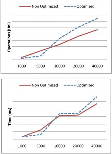
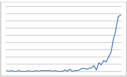
The Y-axis represents time in ms and X relates to the number of binary vectors previously stored in memory. This can be explained because the number of ones in correlated memory is higher than uncorrelated. If you compare this experiment with the coefficient 2, you can see a small decrease in the number of operations (see figure 44).

As expected, as the number of ones in the pictures decreases, associative memory becomes scarcer. 3 Distribution of ones in high-dimensional memory after storage of 200 images with fifty percent ones.

HIERARCHICAL ASSOCIATIVE MEMORY RESULTS

T EST RESULTS ( NO CORRELATION )

The experiments were done by trying to recall patterns from memory that were not previously stored. This means that both the input pattern and the associative memory will be reduced from 1000 units to 500 units. As can be seen, there is a speed up when the query is executed in the aggregated associative memory before the normal one.

In this regard, the following section presents the weight matrix diagram of memory and its distribution according to the methods described in Chapter IV.

A SSOCIATIVE MEMORY DIAGRAMS ( NO CORRELATION )

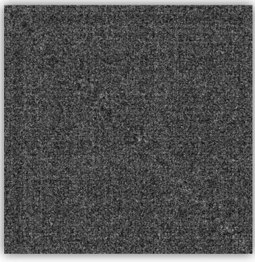
Figure 21 clearly shows that the ones are evenly distributed over the memory. These diagrams and distributions indicate that the datasets have been correctly generated and stored; and that associative memory behaves as it should. It is also important to understand that as the coefficient gets higher, the probability of finding a match in associative memory also increases.

Others go through the different steps until a similar pattern is returned in the last step. The results indicate that there is potential in applying this method before the question is presented to normal associative memory.

T EST RESULTS ( WITH CORRELATION )

As expected, the higher the stacking factor, the smaller the number of operations performed. The objective of combining aggregations in different steps is to reduce the execution time. As can be seen in Figure 27, a three-step aggregation process appears to be ideal when compared to executing each aggregation step individually.

39 higher in the optimized associative memory, since both the aggregated and non-aggregated steps will be performed. It should be noted that a comparison between the correlated and uncorrelated experiment, for the 1000 and 5000 size vector tests, indicates that the execution time decreased.

A SSOCIATIVE MEMORY DIAGRAMS ( CORRELATION )

From this snapshot, we conclude that the datasets used in the experiment are too large. When the memory is full, the tests will not be accurate because the full memory will always return false samples during the recall phase. As we can see in the results below (see Figure 36), the higher clustering is expected to find a similar pattern sooner than the smaller clustering.

In larger datasets with 40000 vectors, each step is processed because a matching pattern is always found. The results lead to the conclusion that for a square associative memory of size 1000, the number of binary vectors correlated in the current experiment is too large.

T EST RESULTS ( WITH CORRELATION AND SMALLER DATA SETS )

The following section presents the weight matrix diagram and distribution of associative memory after storage and 2000 binary vectors with correlation.

A SSOCIATIVE MEMORY DIAGRAMS ( CORRELATION AND SMALLER DATA SETS )

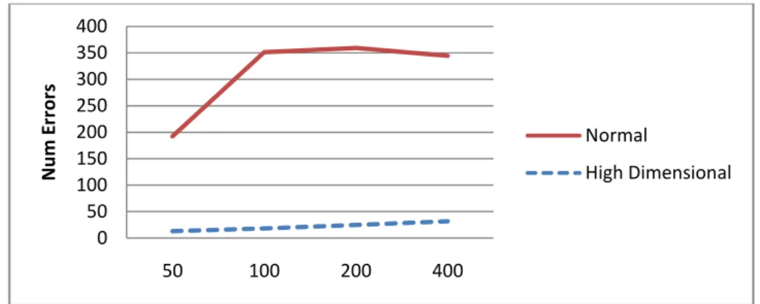
It is important to mention that during the experiments it was found that a small part of the high-dimensional space is not used. Assuming that each one is distributed across the length of the vector, it is safe to assume that the number of ones in the high-dimensional space B, whatever the chosen window size l, is. As was demonstrated in Chapter VI, the number of errors after recalling a non-sparse pattern is several times lower if a high-dimensional space is used instead of the normal one.

Verify high dimensional memory: This option will allow to verify the current units of the high dimensional associative memory. Create a high-dimensional image: Similar to the option above, create a weight matrix diagram of the high-dimensional memory.

EFFICIENT SPARSE CODE RESULTS

C OMMON ASSOCIATIVE MEMORY DIAGRAMS

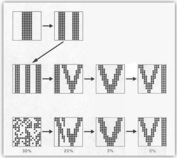
With only thirty percent ones and a data set of fifty images, the diagram indicates that although the memory is not completely full, it is still overloaded and every search results in an incorrect match (see Appendix D.4). The diagrams and distributions related to the 100, 200 and 400 datasets indicate a full memory similar to Figure 47 and Appendix D.4 and will therefore not be repeated. The results for 50 images with ten percent ones show normal distribution and behavior (see Figure 49).

As can be seen from the information gathered in this chapter, data must be sparse to be used in Lernmatrix. The scenario presented in Appendix D.9 and Figure 47 confirms why non-sparse data cannot be used with associative memory.

The 55-dimensional space represents a smaller number of errors, which steadily increases as the number of stored samples increases. 52 Number of errors in high-dimensional and normal associative memories by 30 percent. 53 Number of errors in high-dimensional and normal associative memories by 20 percent.

The results show that the error rate for both memories is similar when neither is full. 54 Number of errors in both high-dimensional and normal associative memories for 10 percent.

It is important to find out when the high dimensional space memory becomes full.

A SSOCIATIVE MEMORY WITH HIGH DIMENSIONAL SPACE DIAGRAMS

To discover this, a second group of data sets was created, larger than the previous ones. To maintain the same ratio between the number of images and unit size, it was decided to reduce the number of images from the previous experiment. By looking carefully at the weight matrix diagram of Appendix D.6 and comparing it with the previous diagram (see Appendix D.5), it can be concluded that both exhibit similar behavior although the current diagram illustrates a sparser memory.

After some consideration, it is possible to explain the behavior illustrated in the previous tests. 59 The results indicate that, similar to what happened in the previous experiments, the space around the diagonal is unused.

C ONCLUSION

CONCLUSION

F UTURE WORK

Regarding the efficient sparse code method, it is important in the mathematical field to find a way to calculate the optimal window size depending on the sparsity of data and size. It would also be interesting to optimize the encoding mechanism to use the entire high-dimensional space. Also, it is important to remember that all the tests were performed with randomly generated binary images.

61 There are not many applications of Lernmatrix in office databases, mainly because of the high requirements regarding the sparsity factor in each input sample.

P ERSONAL C ONTRIBUTIONS

The output of the random image generator is a file containing in the first line the number of images and size followed by each image. Verify Current Memory: This option allows you to verify the state of the associative memory. The duration and number of operations are self-explanatory parameters and represent the execution time of the query and the number of operations required.

Create Image Normal: Create a weight matrix diagram of the memory, similar to the one presented below. Load high dimensional memory: The creation and subsequent storage of patterns in the high dimensional memory is done by this option. Verify memory: As in the previous application, the verify memory option presents the units of the associative memory as a list.

Use Image High Dimensional: Through this option the user can recall a single pattern from the high dimensional associative memory.

BIBLIOGRAPHIC REFERENCES

APPENDIX A

APPENDIX B

APPENDIX C

APPENDIX D

D ISTRIBUTION OF ONES IN THE HIGH DIMENSIONAL MEMORY AFTER STORING 50 IMAGES WITH FIFTY PERCENT ONES

D ISTRIBUTION OF ONES IN THE HIGH DIMENSIONAL MEMORY AFTER STORING 50 IMAGES WITH THIRTY PERCENT ONES

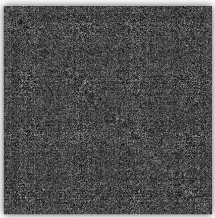
S NAPSHOT OF THE MEMORY AFTER THE STORAGE OF 1000 IMAGES WITH NO CORRELATION

S NAPSHOT OF THE MEMORY AFTER THE STORAGE OF 100 IMAGES WITH CORRELATION

S NAPSHOT OF THE MEMORY AFTER THE STORAGE OF 50 IMAGES WITH 30 PERCENT ONES

S NAPSHOT OF THE HIGH DIMENSIONAL MEMORY AFTER THE STORAGE OF 800 IMAGES WITH 50 PERCENT ONES

S NAPSHOT OF THE HIGH DIMENSIONAL MEMORY AFTER THE STORAGE OF 64 IMAGES WITH 50 PERCENT ONES

S NAPSHOT OF THE MEMORY AFTER THE STORAGE OF 5000 IMAGES WITH NO CORRELATION

T ABLE WITH DATA FOR AGGREGATION 2 AND UNIT SIZE 1000 ( NO CORRELATION / OPTIMAL M VALUE )

T ABLE WITH DATA FOR THREE STEP AGGREGATION (25, 10,5) AND UNIT SIZE 1000 ( NO CORRELATION / OPTIMAL M VALUE )

T ABLE WITH DATA FOR AGGREGATION 2 AND UNIT SIZE 1000 ( WITH CORRELATION / OPTIMAL M VALUE )

T ABLE WITH DATA FOR THREE STEP AGGREGATION (25, 10,5) AND UNIT SIZE 1000 ( WITH CORRELATION / OPTIMAL M VALUE )

T ABLE WITH DATA FOR AGGREGATION 2 AND UNIT SIZE 1000 ( WITH CORRELATION / M VALUE BELOW OPTIMAL )

T ABLE WITH DATA FOR THREE STEP AGGREGATION (25, 10,5) AND UNIT SIZE 1000 ( WITH CORRELATION / M VALUE BELOW OPTIMAL )

T ABLE WITH DATA FOR THREE STEP AGGREGATION (25, 10,5) AND UNIT SIZE 1000 ( WITH CORRELATION / OPTIMAL M VALUE )