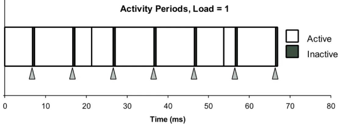
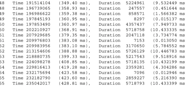
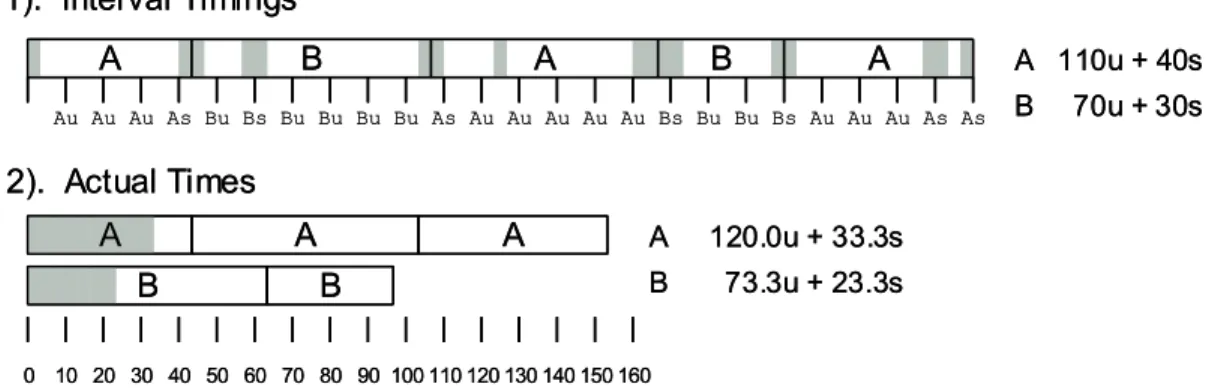
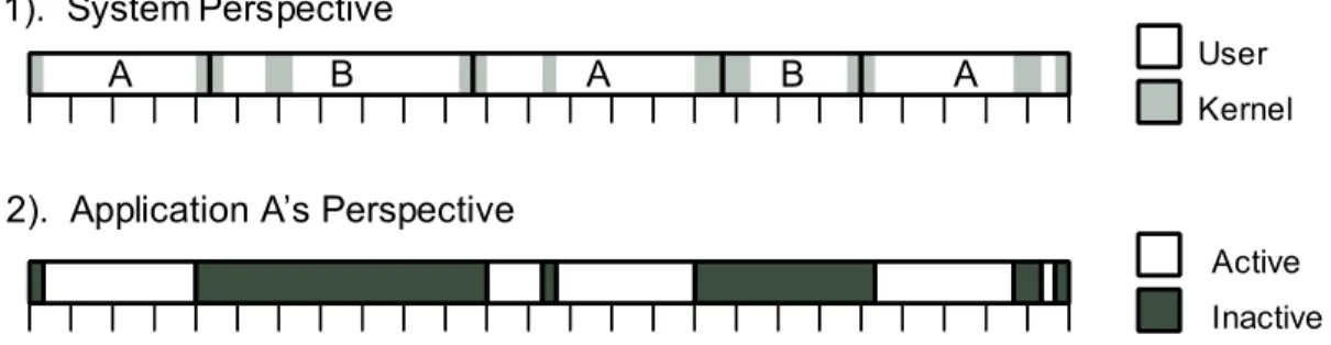
Observe the regular spacing of the boundaries between the periods of activity indicated by the black triangles. Note that the time scales do not match, as the part of the trace we show in Figure 5 started at 349.4 ms into the tracing process. The operating system maintains counts of the amount of user time and the amount of system time used by each process.
When a timer interrupt occurs, the operating system determines which process was active and increments one of the counters for that process by the timer interval. The core activity caused by the timer interrupt takes up - of the total CPU cycles, but these cycles are not properly accounted for.
4 Cycle Counters
IA32 Cycle Counters
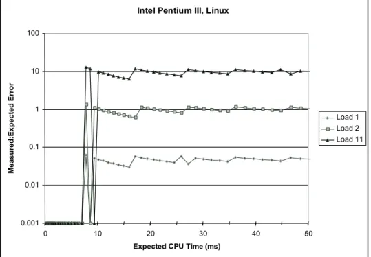
The graphs show our measurements of the error rate, defined as the value of as a function of. The sequence labeled "Load 1" shows the case where the process performing the sampling calculation is the only active process. In general, only measurements that are within the true value are acceptable, so we only want errors of around.
Below about 100ms (10 timer intervals) the measurements are not accurate at all due to the granularity of the timing method. Also note that the errors have a positive bias; the average error for all measurements with ms is 1.04, due to the fact that the timer interrupts take up about 4% of the CPU time. These experiments show that the process hours are only useful for getting approximate values of program performance.
It sets register %edx to the high order 32 bits of the counter and register %eax to the low order 32 bits. This procedure must set the location in the high-order 32 bits of the counter and in the low-order 32 bits. We can use the loop counter to generate activity traces as shown in Figures 3 and 5.
This function continuously checks the cycle counter and detects when two consecutive readings differ by more than the threshold cycles, an indication that the process has been inactive.
5 Measuring Program Execution Time with Cycle Counters
The Effects of Context Switching
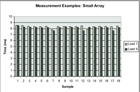
This is especially a problem if the machine is heavily loaded or if the zaP operating time is particularly long. The string labeled "Load 1" indicates runtimes on a lightly loaded machine where it is the only process actively running. The string labeled "Load 4" indicates runtimes when 3 other processes are also running that are heavily using the CPU and memory system.
Caching and Other Effects
The time to execute a block of code can depend heavily on whether the data and instructions used by that code are present in the data and instruction caches at the start of execution. The data locations being updated (labeled b1,b2, alib3.) Let be the number of cycles for this. One problem is that the measurements are not even consistent from one to the next.
As a result, the time to load the code into the instruction cache will be relatively trivial. Executing Ponce before starting the measurement will have the effect of bringing the code used by Pin into the instruction cache. The above code also minimizes the effects of missing the data cache, since the first execution of P will also have the effect of bringing the data accessed by Pinto into the data cache.
To force the timing code to measure the performance of a procedure where none of the data is initially cached, we can clear the cache of all usable data before taking the actual measurement. It stores both values in the dummy and reads them back so that it is cached regardless of the cache allocation policy. It performs a calculation using array values and stores the result in a global integer (the volatile declaration specifies that every update of this variable should be performed), so a smart optimizing compiler will not optimize this part of the code.
The cache flush process also flushes a large portion of the execution stack from the cache, resulting in an overestimation of the time required by the more realistic Punder conditions.
The -Best Measurement Scheme
- Experimental Evaluation
- Setting the value of
- Compensating for Timer Interrupt Handling
- Evaluation on Other Machines
- Observations
A challenge in designing such an experiment is knowing the actual execution time of the programs we are trying to measure. Thus, our scheme can be used to measure relatively short execution times even on a heavily loaded machine. Beyond that, we encounter a systematic overestimation of about 4–6% in a light-load machine and very poor results in a heavy-load machine.
They are consistent with the trace shown in Figure 3, which shows that even on a lightly loaded machine, the application program can only run 95-96% of the time. In our previous experiments, we arbitrarily chose a value of 3 for the parameter, thereby determining the number of measurements we require to be within a small factor of the fastest to finish. It would be a good idea to remove this bias by subtracting an estimate of the time spent handling timer interrupts from the measured program execution time.
To maintain the property of never underestimating the execution time of the procedure, we must set the . As the figure illustrates, we can now get very accurate (within) measurements on a lightly loaded machine, even for programs running multiple time intervals. On this system we were able to get more accurate measurements even for programs with longer run times, especially on lightly loaded machines.
This experiment shows that the internal details of the operating system can greatly affect system performance and our ability to obtain accurate measurements. On a heavily loaded machine, only programs with a duration of less than about 10 ms can be accurately measured. What is the expected number of trials required so that 3 of them are reliable measurements of the procedure, i.e. each performed within a single process segment.
6 Time of Day Measurements
These experiments demonstrate that the -best measurement scheme works reasonably well on a variety of machines. The function writes the time into a structure passed by the caller, which includes one field in units of seconds, and another field in units of microseconds. This is the standard reference point for all Unix systems.] Note that the second argument to gettimeofdays must simply be NULL on Linux systems, as it refers to an unimplemented feature for performing timezone correction.
As shown in Figure 18, we can use gettimeofday to create a pair of launch timer functions and get timers that are similar to our loop time functions, except that the time is measured in seconds rather than clock cycles. Although the fact that the function generates a measurement in units of microseconds seems very promising, it turns out that the measurements are not always that accurate. We define the resolution of the function to be the minimum time value that the timer can resolve.
In the former case, the resolution can be very high - potentially higher than the 1 microsecond resolution provided by the data representation. In the latter case, the resolution will be poor - no better than what is provided by functionstimesandclock. We calculated this by calling the function repeatedly until one second had passed and dividing 1 by the number of calls.
We show results on two different machines to illustrate the effect of time resolution on accuracy.
7 Concluding Observations
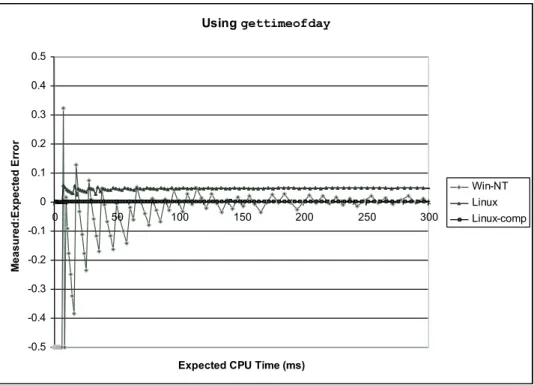
As can be seen, this function requires about 1 microsecond on most systems and a few microseconds on others. The measurements on a Windows NT system show characteristics similar to those we found for Linux using times (Figure 8.) Since gettimeofday is implemented using the process timers, the error can be negative or positive and is mainly erratic for short duration measurements. Accuracy improves over time, to the point where the error is less than .
This can be seen by comparing the measurements with the results of Load 1 in Figure 12 (without compensation) and in Figure 14 (with compensation.) Using compensation we can achieve better than accuracy, even for measurements up to 300ms. Details about the implementation of the operating system and library function can have a significant effect on what kinds of programs can be measured and with what accuracy. This leads to the compensation scheme that greatly improves accuracy on a lightly loaded Linux system.
Given the variations from one system to another, and even from one OS kernel release to another, it's important to be able to analyze and understand the many aspects of a system that affect its performance. It is relatively easy for the operating system to manage the cycle counter to show the number of cycles passed for a specific process. Then, when the process is reactivated, the loop counter is set to the value it had when the process was last deactivated, effectively freezing the counter while the process is inactive.
In an effort to reduce power consumption, future systems will vary the clock speed, as power consumption is directly proportional to the clock speed.
A Solution to Problems
- Solution
- Solution
- Solution
- Solution
- Solution
- Solution
- Solution
- Solution
- Solution
- Solution
For the minimal case, the segment started just before the time 10 timeout and ended just as the time 70 timeout occurred, giving a total time of just over 60 ms. For the maximal case, the segment started immediately after the time 0 timeout and continued until just before the time 80 timeout, giving a total time of just under 80 ms. In the actual trace, the process took 63.7 ms in user mode and 3.3 ms in kernel mode.
If the call to sleep occurs just after a timer interrupt, the process will be inactive for almost exactly 2 seconds. If it occurs just before a timer interrupt, then it will be inactive for just 1.99 seconds, give.