The calibration of the diode laser detuning is obtained with saturated absorption spectroscopy (upper curve). The Rabi frequency of the input laser is Ωa= Ωb=0.1Γ. b) Frequency of the oscillation in the correlation function of (a).
Energy structure of alkali atoms
In the latter case, the existence of the electron spin leads to the spin-orbit (SO) interaction, which is described by the Hamiltonian [44]. The splitting power of this energy structure depends on the nuclear spin of the element and the energy level of the electron.
Electromagnetic fields
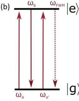
With such polarization, a fourth photon is generated in the frequency of the FWM process to conserve energy and momentum. Another common configuration for the FWM process is the so-called degenerate configuration, in which all the incident fields are at the same frequency.
Bloch equations
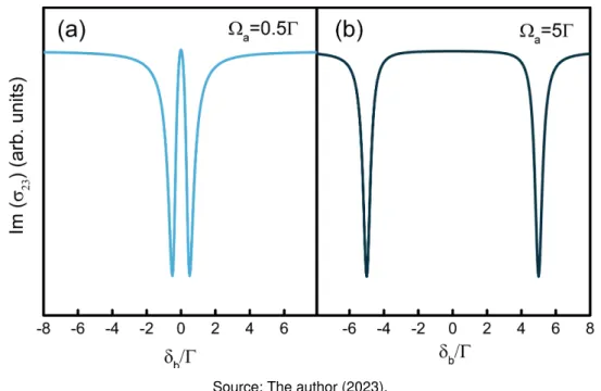
At this point we introduce slow system variables to eliminate explicit time dependence later. 5(b), we increased the Rabi frequency of the control field by a factor of ten, resulting in a completely different transmission curve.

Optical pulse train
We obtain the CBL signal by scanning the cw laser frequency or repetition rate of the pulsed laser. One of the key features of mode-locked lasers occurs in the frequency domain, as they generate a series of equal frequency components, known as a frequency comb.

CBL experimental setup
7 we show that part of the light from the diode laser is fed to a saturated absorption spectroscopy (SAS) experiment. It is crucial to monitor the frequency of the diode laser, and to do so we use the results from SAS.

Autler-Townes splitting
As the strength of the strong field increases, a doublet structure is observed in the results shown in the figure. The distance between the peaks also depends on the power of the diode laser. 10 is a frequency separation of hundreds of MHz, while the Rabi frequency of a diode laser (strong field) is only tens of MHz.
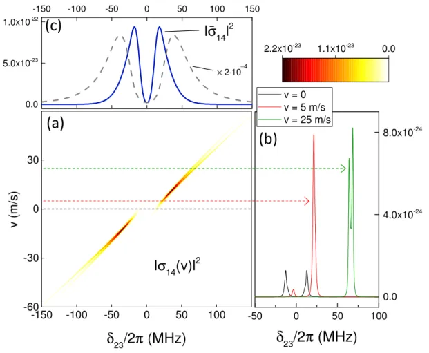
We will show in the theoretical subsection that even a small detuning can change the symmetry of the FWM signal. In this four-plane case, the matrix representation of the hamiltonian is Hˆ in the rotating frame. As in the experiment, we consider two frequency scanning scenarios, where either the frequency of the weak beam (Ω23) or the frequency.
Now consider an increase in the Rabi frequency of the field in the lower transition (|1i → |2i). This results in the peak amplitude as a function of the strong beam Rabi frequency shown in Fig.

Interference between excitation pathways
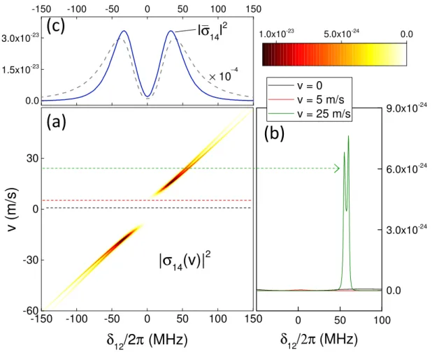
Another feature we highlighted in the experimental results was the frequency separation between the peaks of the signal or the "splitting" of the doublet. Once again, if we consider the system to be open due to the high intensity of the strong field, these results improve, as shown in Fig. In this scenario we are interested in the frequency scanning scheme where the repetition rate of fs laser varies while diode laser has a fixed frequency.
In this graph, we present the curves for three different values of the diode laser intensity, showing the doublet structure due to the dynamic Stark shift with the characteristics we discussed before. This narrow peak is observed depending on the value of the repetition rate, and a close-up of the doublet structure on the right side of the curve (II) is shown in the upper curve of Fig. The linewidth of the observed narrow interference peak, of about 10 MHz, is mainly limited by experimental conditions such as the repetition rate scan.
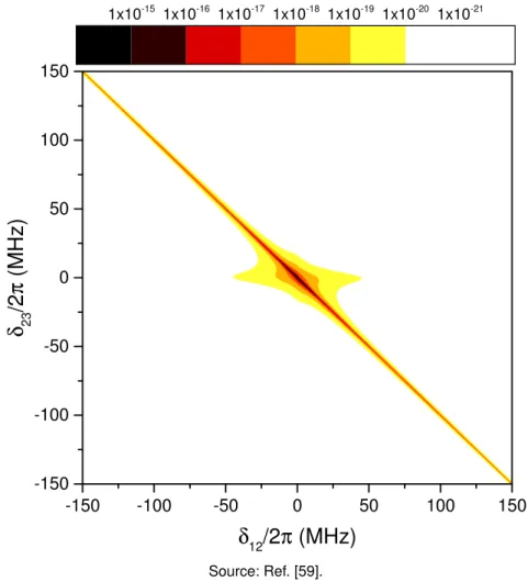
In contrast, the theoretical model shows that the peak has a linewidth of about 1 MHz, a result that seems to be related to the lifetime of the 5D5/2state [93]. The theoretical results indicate that to correctly describe the frequency position of each peak, we need to solve the Bloch equations, including higher order terms.

Experimental setup and results
Moreover, these peaks only appear in the spectra due to the simultaneous interaction of the two incident fields with the atomic medium. We present one of the transmission curves and the two corresponding FWM signals in Fig. In this case, the ratio between the intensities of the incident rays is ≈3, with Eabeing stronger.
27(a), we scan the frequency of the field EawhileEb has a fixed frequency and vice versa for Fig. Insets, zoom of the peak corresponding to the cyclic transition on the Ta curve in each measurement. This absorption dip occurs in the middle of the two nonlinear signals, indicating that both lasers resonate with the closed transition.
There is also a drop in EIA at the other two peaks of the transmission curves, although they are considerably smaller. To obtain these measurements, we scan the frequency of one of the fields (Ea) while keeping the frequency of the other field (Eb) fixed.
Theoretical model
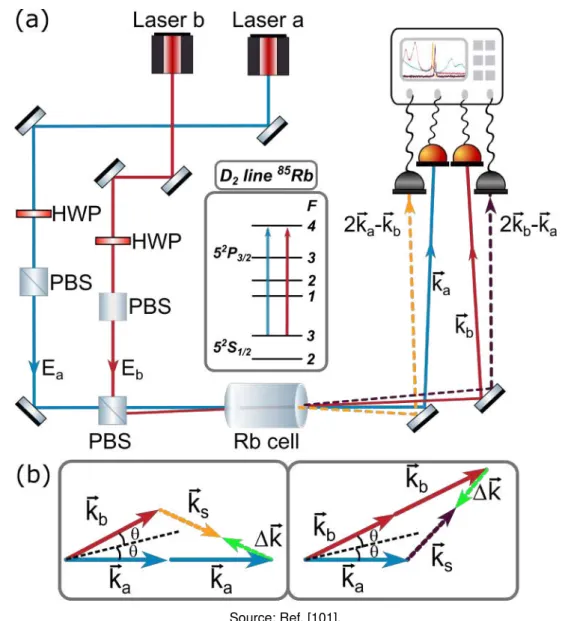
As the input laser intensity increases, we observe a power broadening effect on the FWM signals, as well as an increase in the frequency separation between them. For example, if one chooses the direction of polarization of one of the input beams as the quantization axis. With the complete set of solutions of the Bloch equations, we write the coherences σ210 and σ230.
The polarization P can be written in terms of a complex amplitude that oscillates with the frequency of the field. The refractive index as a function of the Ea field is shown in Fig. This is a feature seen in the EIA process [104], which is observed in the transmission of input beams.
The modeling of the refractive index is crucial for reproducing the characteristics of the experimental signal. In the previous section, we modeled results related to the inhomogeneous broadening of the atomic medium.

Magneto-Optical Trap
The power in this case is given by the multiplication of the photon momentum and the scattering rate. In this scheme, called magneto-optical trap, we add some coils in the anti-Helmholtz configuration to the experimental setup of the optical molasses, that is, there is a new term, a restoring force, which means that the dynamics of the atoms in the trap follows a harmonic motion, typically overdamped [44].
In the optical setup of the experiment, we use two diode lasers of the same type as in the previous sections (Sanyo DL7140-201S). Since there are many optical elements in the path of the cooling beam before it reaches the atoms, considerable power is lost. MOT can be observed with an IR camera due to the spontaneously emitted light produced by the hunting process.
The same fluorescence that allows the CCD to capture images of the cloud could be used to measure the number of atoms. The diameter of the MOT and the number of atoms are part of several parameters that can be obtained from characterization measurements [119].

Experimental setup and results
The two FWM signals and the transmissions of the input beams a and b are detected by avalanche photodiodes (APD) of the models APD120A/M (max responsivity at 800 nm) and APD120A2/M (max responsivity at 600 nm) from Thorlabs. The signal we are interested in now is the time series of the intensity fluctuations for all four signals and the two polarizations. The intensity fluctuations of the four signals and their two polarizations are shown in Figure 44.
Time series of the intensity fluctuations of the transmittance of the input lasers with Ia=Ib=0.15mW/cm2,δ/2π=15MHz and (c) circular and parallel polarizations;. 44, that there is a strong temporal positive correlation in the intensity fluctuations of the output signals. In particular, these curves are remarkably similar to the cross-correlation (dark brown curves) of the two transmission signals.
The most notable feature is that the correlation curves become broader as the frequency of the input laser approaches resonance. 49, the Fourier transform of the second-order correlation function of transmission signals (see Fig. 47).

Theoretical model
In this model, they perform a Floquet expansion of the density matrix elements in the frequency of the input fields and their combinations. This is in contrast to a simple random walk, where the variance of the system grows indefinitely over time. Degenerate four-wave mixing with cold atoms: intensity correlations 129. The results do not differ drastically as long as the variance of the process, given by β2/2α, is small.
Once the numerical simulation is complete, we can use the time series of the density matrix elements to calculate the second-order correlation function for the intensity fluctuations. This means that in the first-order approximation we perceive a superposition of the input and generated fields. To calculate the second-order correlation function of intensity fluctuations, we can rewrite the equation.
It shows a broadening of the correlation peak that is compatible with the behavior of the experimental result. Moreover, the theoretical results highlight the oscillation of the correlation curve in the generalized Rabi frequency.
Analysis of the FWM spectra
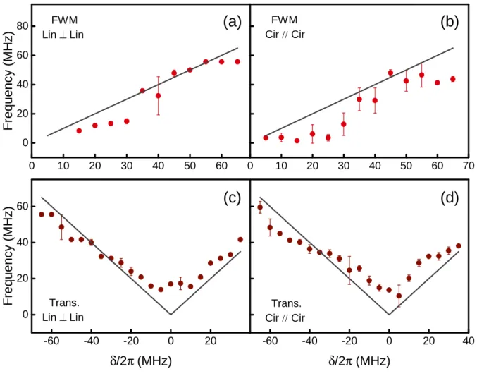
Therefore, the Rabi frequencies of the input fields and the FWM field are given by the coupled equations. This implies that there is a non-absorption resonance for δ = 0 [54] due to the transverse optical pumping of the population. The asymmetry of the experimental results is not present in the model, but as we discussed before, it is connected to the frequency scan rate.
On the other hand, the theoretical solution does not agree with the experiment for higher intensities of the input lasers. 53], in which the authors perform a Floquet expansion of the density matrix elements in the frequency of the input fields and their combinations. 38] which provides an anti-relationship between FWM signals due to the non-degeneracy of the ground conditions.
Measurement of the electric dipole moments for transitions to rubidium rydberg states via Autler-Townes splitting. Conditions for the observation of the Autler-Townes effect in a two-step resonance experiment.Journal de Physique, v.