III Economic Impacts of COVID-19

(1)

How Did COVID-19 and Stabilization Policies Affect Spending and Employment?

A New Real-Time Economic Tracker Based on Private Sector Data

^∗

Raj Chetty, John N. Friedman, Nathaniel Hendren, Michael Stepner, and the Opportunity Insights Team^†

June 17, 2020

Abstract

We build a publicly available platform that tracks economic activity at a granular level in real time using anonymized data from private companies. We report weekly statistics on consumer spending, business revenues, employment rates, and other key indicators disaggregated by county, industry, and income group. Using these data, we study the mechanisms through which COVID-19 affected the economy by analyzing heterogeneity in its impacts across geographic areas and income groups. We first show that high-income individuals reduced spending sharply in mid-March 2020, particularly in areas with high rates of COVID-19 infection and in sectors that require physical interaction. This reduction in spending greatly reduced the revenues of businesses that cater to high-income households in person, notably small businesses in affluent ZIP codes. These businesses laid off most of their low-income employees, leading to a surge in unemployment claims in affluent areas. Building on this diagnostic analysis, we use event study designs to estimate the causal effects of policies aimed at mitigating the adverse impacts of COVID. State-ordered reopenings of economies have little impact on local employment. Stim- ulus payments to low-income households increased consumer spending sharply, but had modest impacts on employment in the short run, perhaps because very little of the increased spending flowed to businesses most affected by the COVID-19 shock. Paycheck Protection Program loans have also had little impact on employment at small businesses. These results suggest that traditional macroeconomic tools – stimulating aggregate demand or providing liquidity to businesses – may have diminished capacity to restore employment when consumer spending is constrained by health concerns. During a pandemic, it may be more fruitful to mitigate economic hardship through social insurance. More broadly, this analysis illustrates how real-time economic tracking using private sector data can help rapidly identify the origins of economic crises and facilitate ongoing evaluation of policy impacts.

∗We thank Gabriel Chodorow-Reich, Jason Furman, Xavier Jaravel, Lawrence Katz, Emmanuel Saez, Ludwig Straub, and Danny Yagan for helpful comments. We also thank the corporate partners who provided the underlying data used in the Economic Tracker, who as of this version include: Affinity Solutions (especially Atul Chadha and Arun Rajagopal), Burning Glass (especially Anton Libsch and Bledi Taska), Earnin (especially Arun Natesan and Ram Palaniappan), Homebase (especially Ray Sandza and Andrew Vogeley), Intuit (especially Christina Foo and Krithika Swaminathan), Womply (especially Toby Scammell and Ryan Thorpe), and Zearn (especially Billy McRae and Shalinee Sharma). We are very grateful to Ryan Rippel of the Gates Foundation for his support in launching this project and to Gregory Bruich for early conversations that helped spark this work. The work was funded by the Chan-Zuckerberg Initiative, Bill & Melinda Gates Foundation, Overdeck Family Foundation, and Andrew and Melora Balson. The project was approved under Harvard University IRB 20-0586.

†The Opportunity Insights Economic Tracker Team consists of Matthew Bell, Gregory Bruich, Tina Chelidze, Lucas Chu, Westley Cineus, Sebi Devlin-Foltz, Michael Droste, Shannon Felton Spence, Dhruv Gaur, Federico Gonza- lez, Rayshauna Gray, Abby Hiller, Matthew Jacob, Tyler Jacobson, Margaret Kallus, Laura Kincaide, Cailtin Kupsc, Sarah LaBauve, Maddie Marino, Kai Matheson, Kate Musen, Danny Onorato, Sarah Oppenheimer, Trina Ott, Lynn Overmann, Max Pienkny, Jeremiah Prince, Daniel Reuter, Peter Ruhm, Emanuel Schertz, Kamelia Stavreva, James Stratton, Elizabeth Thach, Nicolaj Thor, Amanda Wahlers, Kristen Watkins, Alanna Williams, David Williams, Chase Williamson, Shady Yassin, and Ruby Zhang.

(2)

I Introduction

Since the pioneering work of Kuznets (1941), macroeconomic policy decisions have been made on the basis of data collected from recurring surveys of households and businesses conducted by the federal government. Although such statistics have great value for understanding the economy, they have two limitations that have become apparent during the COVID-19 pandemic. First, such data are typically available only at a low frequency with a significant time lag. For example, disaggregated quarterly data on consumer expenditures are typically available with a one year lag in the Consumer Expenditure Survey (CEX). Second, such statistics typically cannot be used to assess granular variation across geographies or subgroups; due to limitations in sample sizes, most statistics are typically reported only at the national or state level and breakdowns by subgroups or sectors are often unavailable.

In this paper, we address these challenges by building a new, freely accessible platform that tracks economic activity at a high-frequency, granular level using anonymized and aggregated data from private companies. Combining data from credit card processors, payroll firms, and financial services firms, we construct statistics on consumer spending, employment rates, business revenues, job postings, and other key indicators described in detail in Section II below. We report these statistics in real time using an automated pipeline that ingests data from businesses and reports statistics publicly on the data visualization platform, typically less than seven days after the relevant transactions occur. We present fine disaggregations of the data, reporting each statistic by county and by industry and, where feasible, by initial (pre-crisis) income level and business size.

Many firms already analyze their own data internally to inform business decisions and some firms have begun sharing aggregated data with policymakers and researchers during the current crisis.

Our contribution is to (1) combine these disparate data sources into a single, publicly accessible platform that eliminates the need to write contracts with specific companies to access relevant data;

(2) systematize these data sources by documenting the samples they cover and benchmarking them to existing public series; and (3) provide the combined series in an interactive data visualization tool that facilitates comparisons across outcomes, areas, and subgroups.

Unlike official government statistics, which are based on sampling frames designed to provide representative information, our statistics reflect the behavior of the clients of the firms from which we obtain data. To mitigate selection biases that can arise from this approach, we use data from companies that have large samples (e.g., at least one million individuals), span well-defined sectors

(3)

or subgroups (e.g., small businesses, bottom-income-quintile workers), and track publicly available benchmarks in historical data. Although there is no guarantee that the statistics from such data sources capture total economic activity accurately, we believe they contain useful information because the shocks induced by major crises such as COVID-19 are large relative to plausible biases due to non-representative sampling, as shown e.g. by Cajner et al. (2020) in the context of payroll data and Dunn, Hood, and Driessen (2020) in the context of spending data.

We use these new data to analyze the economic impacts of the coronavirus pandemic (COVID- 19). Government statistics show that COVID led to a very sharp reduction in GDP and an unprecedented surge in unemployment. Our goal is to understand the factors that led to these macroeconomic changes by disaggregating these statistics across subgroups and areas.

National accounts data reveal that most of the reduction in GDP came from a reduction in consumer spending (rather than business investment, government purchases, or exports). We therefore begin our analysis by examining the drivers of changes in consumer spending, focusing in particular on credit and debit card spending. We first establish that card spending closely tracks historical benchmarks on retail spending and services, which together constitute a large fraction of the reduction in total spending in the national accounts. We then show that the vast majority of the reduction in consumer spending in the U.S. came from reduced spending by high-income households. As of June 10, more than half of the total reduction in card spending since January had come from households in the top quartile of the income distribution; only 5% had come from households in the bottom income quartile.¹ This is both because the rich account for a larger share of total spending to begin with and because high-income households reduced their spending by 17%, whereas low-income households reduced their spending by only 4% as of June 10.

Most of the reduction in spending is accounted for by reduced spending on goods or services that require in-person physical interaction and thereby carry a risk of COVID infection, such as hotels, transportation, and food services, consistent with the findings of Alexander and Karger (2020). The composition of spending cuts – with a large reduction in services – differs sharply from that in prior recessions, where service spending was essentially unchanged and durable goods spending fell sharply. Zooming into specific subcategories, we find that spending on luxury goods

1. We impute income as the median household income (based on Census data) in the cardholder’s ZIP code. We verify the quality of this imputation procedure by showing that our estimates of the gap in spending reductions by income group are aligned with those of Farrell et al. (2020), who observe income directly for JPMorgan Chase clients, as of mid-April 2020, the last date available in their series. We find that spending levels of low-income households increased much more sharply than those of high-income households since mid-April largely as a result of stimulus payments.

(4)

that do not require physical contact – such as landscaping services or home swimming pools – did not fall, while spending at salons and restaurants plummeted. Businesses that offer fewer in person services, such as financial and professional services firms, also experienced much smaller losses.

The fact that spending fell in proportion to the degree of physical exposure required across sectors suggests that the reduction in spending by the rich was driven primarily by health concerns rather than a reduction in income or wealth. Indeed, the incomes of the rich have fallen relatively little in this recession (Cajner et al. 2020). Consistent with the centrality of health concerns, we find that the reductions in spending and time spent outside home were larger in high-income, high- density areas with higher rates of COVID infection, perhaps because high-income individuals can self-isolate more easily (e.g., by substituting to remote work). Together, these results suggest that consumer spending in the pandemic fell because of changes in firms’ ability to supply certain goods (e.g., restaurant meals that carry no health risk) rather than because of a reduction in purchasing power.²

Next, we turn to the impacts of the consumer spending shock on businesses. To do so, we exploit the fact that many of the sectors in which spending fell most are non-tradable goods produced by small local businesses (e.g., restaurants) who serve customers in their local area. Building on the results on the heterogeneity of the spending shock, we use differences in average incomes and rents across ZIP codes as a source of variation in the spending shock that businesses face. This geographic analysis is useful both from the perspective of understanding mechanisms and because prior work shows that geography plays a central role in the impacts of economic shocks due to low rates of migration that can lead to hysteresis in local labor markets (Austin, Glaeser, and Summers 2018, Yagan 2019).

Small business revenues in the most affluent ZIP codes in large cities fell by more than 70%

between March and late April, as compared with 30% in the least affluent ZIP codes. These reductions in revenue resulted in a much higher rate of small business closure in high-rent, high- income areas within a given county than in less affluent areas. This is particularly the case for non-tradable goods that require physical interaction – e.g., restaurants and accommodation services – where revenues fell by more than 80% in the most affluent neighborhoods in the country, such as the Upper East Side of Manhattan or Palo Alto, California. Small businesses that provide fewer

2. This explanation may appear to be inconsistent with the fact that the Consumer Price Index (CPI) shows little increase in inflation, given that one would expect a supply shock to increase prices. However, the CPI likely understates inflation in the current crisis because it does not capture the extreme shifts in the consumption bundle that have occurred as a result of the COVID crisis (Cavallo 2020).

(5)

in-person services – such as financial or professional services firms – experience much smaller losses in revenue even in affluent areas.

As businesses lost revenue, they passed the incidence of the shock on to their employees. Low- wage hourly workers in small businesses in affluent areas are especially likely to have lost their jobs.

In the highest-rent ZIP codes, more than 65% of workers at small businesses were laid off within two weeks after the COVID crisis began; by contrast, in the lowest-rent ZIP codes, fewer than 30%

lost their jobs. Workers at larger firms and in tradable sectors (e.g., manufacturing) were much less likely to lose their jobs than those working in small businesses producing non-tradable goods, irrespective of their geographic location. Job postings also fell much more sharply in more affluent areas, particularly for lower-skilled positions. As a result of these changes in the labor market, unemployment claims surged even in affluent counties, which have generally had relatively low unemployment rates in prior recessions. For example, more than 15% of residents of Santa Clara county – the richest county in the United States, located in Silicon Valley – filed for unemployment benefits by May 2. Perhaps because they face higher rates of job loss and worse future employment prospects, low-income individuals working in more affluent areas cut theirown spending much more than low-income individuals working in less affluent areas.

In summary, the initial impacts of COVID-19 on economic activity appear to be largely driven by a reduction in spending by higher-income individuals due to health concerns, which in turn affected businesses that cater to the rich – e.g., small businesses in affluent areas – and ultimately reduced the incomes and expenditure levels of low-wage employees of those businesses. In the final part of the paper, we analyze the impacts of three major policy efforts that were enacted in an effort to break this chain of events and mitigate the economic impacts of the crisis: state-ordered reopenings, stimulus payments to households, and loans to small businesses.

Reopenings of economies had modest impacts on economic activity. Spending and employment remained well below baseline levels even after reopenings, and in particular did not rise more rapidly in states that reopened earlier relative to comparable states that reopened later. Spending and employment also fell wellbefore state-level shutdowns were implemented, consistent with other recent work examining data on hours of work and movement patterns (Bartik et al. 2020, Villas- Boas et al. 2020).

Stimulus payments provided through the CARES Act increased spending among low-income households sharply, nearly restoring their spending to pre-COVID levels as of May 10, consistent with evidence from Baker et al. (2020). Most of this increase in spending was in sectors that require

(6)

limited physical interaction. Purchases of durable goods surged, while consumption of in-person services (e.g., restaurants) increased very little. As a result, very little of the increased spending flowed to businesses most affected by the COVID-19 shock, such as small businesses in affluent areas – potentially limiting the capacity of the stimulus to increase economic activity and employment in the communities where job losses were largest.

Loans to small businesses as part of the Paycheck Protection Program (PPP) also have had little impact on employment rates at small businesses to date. Employment rates at small firms in the hardest-hit sectors trended similarly to those at larger firms that were likely to be ineligible for PPP loans, and remained far below baseline levels as of May 30. These results suggest that providing liquidity itself may be inadequate to restore employment at small businesses, at least in the short run.³

In sum, our analysis suggests that the primary barrier to economic activity is depressed consumer spending due to the threat of COVID-19 itself as opposed to government restrictions on economic activity, inadequate income among consumers, or a lack of liquidity for firms. Hence, the only path to full economic recovery in the long run may be to restore consumer confidence by addressing the virus itself (e.g., Allen et al. 2020, Romer 2020). Traditional macroeconomic tools – stimulating aggregate demand or providing liquidity to businesses – may have diminished short-run impacts in an environment where consumer spending is fundamentally constrained by health concerns.

In the meantime, it may be more fruitful to approach this economic crisis from the lens of providing social insurance to reduce hardship rather than stimulus to increase economic activity.

Rather than attempt to put workers back to work in sectors where spending is temporarily depressed because of health concerns, it may be best to focus on mitigating income losses for those who have lost their jobs, consistent with the normative predictions of the theoretical framework developed by Guerrieri et al. (2020). For instance, providing support to workers who have lost their jobs (e.g., via the unemployment benefit system) may be preferable to stimulus payments to all households, irrespective of their employment situation. Our findings also suggest that may be useful to consider additional place-based assistance targeted at low-income individuals in areas that have suffered the largest losses – such as affluent, urban areas – since historical experience suggests that relatively

3. The PPP also includes price incentives to rehire workers in the form of loan forgiveness for firms that employ the same number of workers as of June 30 as they did in February. Firms may rehire workers in light of this incentive in the coming month, a possibility that can be evaluated in real time using the data in the tracker. What is clear at this stage is that liquidity itself – absent this price incentive or fundamental changes in the public health situation – appears to be insufficient to restore employment to pre-recession levels.

(7)

few people move to other labor markets to find new jobs after recessions (Yagan 2019).

Of course, all of these results could change over time: the recession may turn into a more traditional economic shock with Keynesian spillovers across a wider set of sectors and areas as time passes, in which case tools such as stimulus and liquidity could become much more impactful (Guerrieri et al. 2020). The tracker constructed here can be used to monitor the changing dynamics of the crisis and evaluate policy impacts on an ongoing basis.

Our work builds on and contributes to a rapidly evolving literature on the economic impacts of COVID-19 as well as a long literature in macroeconomics on the measurement of economic activity at business cycle frequencies. Several recent papers have used private sector data analogous to what we assemble here to analyze consumer spending (e.g., Baker et al. 2020, Chen, Qian, and Wen 2020, Farrell et al. 2020), business revenues (e.g., Alexander and Karger 2020), labor market trends (e.g., Bartik et al. 2020, Kurmann, Lal´e, and Ta 2020, Kahn, Lange, and Wiczer 2020), and social distancing (e.g., Allcott et al. 2020, Chiou and Tucker 2020, Goldfarb and Tucker 2020, Mongey, Pilossoph, and Weinberg 2020). These papers have identified a number of important results consistent with our findings, such as concentrated impacts on spending in certain industries such as food and accommodation; social distancing that is a result of voluntary choices rather than legislation; and large employment losses for low-income workers. Each of these papers analyzes a subset of data sources, obtained through a data use agreement with the relevant firm. By combining these and other datasets and benchmarking them to national aggregates, we are able to trace the macroeconomic impacts of the COVID shock from consumer spending to businesses to labor markets. More generally, by integrating these datasets into a unified, freely accessible platform, we eliminate the need to obtain specific permissions to use data from each company.

We hope this platform will provide a prototype for developing real time national accounts based on administrative data held by private companies that can be used to inform and evaluate policy decisions in this crisis and beyond.

The paper is organized as follows. The next section describes the data we use to construct the economic tracker. In Section 3, we analyze the effects of COVID-19 on spending, revenue, and employment. Section 4 analyzes the impacts of policies enacted to mitigate COVID’s impacts.

Section 5 concludes. Technical details on data, methods, and supplementary analyses are available in an online appendix.

(8)

II Data and Methods

We use anonymized data from several private companies to construct indices of spending, employment, and other metrics. In this section, we describe how we construct each series. To facilitate comparisons between series, we adopt the following set of principles when constructing each series (wherever feasible given data availability constraints).

First, the central challenge in using private sector data to measure economic activity is that they capture information exclusively about the customers each company serves, and thus are not necessarily representative of the full population. Instead of attempting to adjust for this non- representative sampling, we characterize the portion of the economy that each series captures by comparing the characteristics of each sample we use to national benchmarks.⁴

Second, we clean each series to remove artifacts that arise from changes in the data providers’

coverage or systems. For instance, firms’ clients often change discretely, sometimes leading to discontinuous jumps in series, particularly in small cells. We systematically search for large jumps in series (e.g., >80%), seek to understand their root causes, and address such discontinuities by imposing continuity as described below.

Third, many series exhibit substantial periodic fluctuations across days. We address such fluctuations through aggregation, e.g. reporting 7-day moving averages to smooth daily fluctuations.

Certain series – most notably consumer spending and business revenue – exhibit strong weekly fluctuations that are autocorrelated across years (e.g., a surge in spending around the holiday season).

We de-seasonalize such series by normalizing each week’s value in 2020 relative to corresponding values for the same week in 2019 in our baseline analysis, but also report raw values for 2020 for researchers who prefer to make alternative seasonal adjustments.

Fourth, to protect confidentiality of business market shares, we do not report levels of the series.

Instead, we report indexed values that show percentage changes relative to mean values in January 2020.⁵ We also suppress small cells and exclude outliers to protect the privacy of individuals and businesses, with thresholds that vary across datasets as described below.

4. An alternative approach is to reweight samples based on observable characteristics – e.g., industry – to match national benchmarks. We do not pursue such an approach here because the samples we work with track relevant national benchmarks – at least for the scale of shocks induced by the COVID crisis – without such reweighting.

However, the disaggregated data we report by industry and county can be easily reweighted as desired in future applications.

5. We always norm after summing to a given cell (e.g. geographic unit, industry, etc.) rather than at the firm or individual level. This dollar-weighted approach overweights bigger firms and higher-income individuals, but leads to smoother series and is arguably more relevant for certain macroeconomic policy questions (e.g., changes in aggregate spending).

(9)

Finally, we seek to release data series at the highest possible frequency. To limit revisions, we permit a sufficient lag to adjust for reporting delays (typically one week). We disaggregate each series by two-digit NAICS industry code; by county, metro area, and state; and by income quartile where feasible.⁶

We now describe each of the series in turn, discussing the raw data sources, construction of key variables, and cross-sectional comparisons to publicly available benchmarks.⁷ All of the data series described below can be freely downloaded from the Economic Tracker website: www.tracktherecovery.org.

II.A Consumer Spending: Affinity Solutions

We measure consumer spending using aggregated and anonymized consumer purchase data collected by Affinity Solutions Inc, a company that aggregates consumer credit card spending information to support a variety of financial service products.

We obtain raw data from Affinity Solutions at the county-by-ZIP code income quartile-by- industry-by-day level starting from January 1, 2019. Industries are defined by grouping together similar merchant category codes. ZIP code income quartiles are constructed at the national level using Census data on population and median household income by ZIP. Cells with fewer than five unique card transactions are masked.

The raw data include several discontinuous breaks caused by entry or exit of credit card providers from the sample. We identify these breaks using data on the total number of active cards in the cell. We then estimate the discontinuous level shift in spending resulting from the break (using a standard regression discontinuity estimator). At the state level (including Washington, DC), we adjust the series within each cell by adding the RD estimate back to the raw data to obtain a smooth series. At the county-level, there is too much noise to implement a reliable correction, so we exclude counties that exhibit such breaks from the sample. After cleaning the raw data in this manner, we construct daily values of the consumer spending series using a seven-day moving average of the current day and previous six days of spending. We then seasonally adjust the series by dividing each calendar date’s 2020 value by its corresponding value from 2019.⁸ Finally, we index the seasonally-adjusted series relative to pre-COVID-19 spending by dividing each day’s value by the mean of the seasonally-adjusted seven-day moving average from January 8-28.

6. We construct metro area values for large metro areas using a county to metro area crosswalk described in the Appendix.

7. We benchmark trends in each series over time to publicly-available data in the context of our analysis in the next section.

8. We divide the daily value for February 29, 2020 by the average value between the February 28, 2019 and March 1, 2019.

(10)

Comparison to QSS and MRTS. Total debit and credit card spending in the U.S. was $7.08 trillion in 2018 (Board of Governors of the Federal Reserve System 2019), approximately 50% of total personal consumption expenditures recorded in national accounts. Affinity Solutions captures nearly 10% of debit and credit card spending in the U.S. To assess which categories of spending are covered by the Affinity data, Appendix Figure 1 compares the spending distributions across sectors to spending captured in the nationally representative Quarterly Services Survey (QSS) and Monthly Retail Trade Survey (MRTS). Affinity has broad coverage across industries. However, as expected, it over-represents categories where credit and debit cards are used for purchases. In particular, accommodation and food services and clothing are a greater share of the Affinity data than financial services and motor vehicles. We therefore view Affinity as providing statistics that are representative of total card spending (but not total consumer spending). We assess whether Affinity captures changes in card spending around the crisis in Section 3.1 below.

II.B Small Business Revenue: Womply

We obtain data on small business transactions and revenues from Womply, a company that aggregates data from several credit card processors to provide analytical insights to small businesses and other clients. In contrast to the Affinity series on consumer spending, which is a cardholder-based panel covering total spending, Womply is a firm-based panel covering total revenues of small businesses. The key distinction is that location in Womply refers to the location where the business transaction occurred as opposed to the location where the cardholder lives.

We obtain raw data on small business transactions and revenues from Womply at the ZIP- industry-day level starting from January 1, 2019.⁹ Small businesses are defined as businesses with annual revenue belowSmall Business Administration thresholds. To reduce the influence of outliers, firms outside twice the interquartile range of firm annual revenue within this sample are excluded and the sample is further limited to firms with 30 or more transactions in a quarter and more than one transaction in 2 out of the 3 months.

We aggregate these raw data to form two publicly available series at the county by industry level:

one measuring total small business revenue and another measuring the number of small businesses open. We measure small business revenue as the sum of all credits (generally purchases) minus debits (generally returns). We define small businesses as being open if they have a transaction in the last three days. We exclude counties with a total average revenue of less than $250,000 during

9. We crosswalk Womply’s transaction categories to two-digit NAICS codes using an internally generated Womply category-NAICS crosswalk, and then aggregate to NAICS supersectors.

(11)

the pre-COVID-19 period (January 4-31).

For each series, we construct daily values in exactly the same way that we constructed the consumer spending series. We first take a seven-day moving average, then seasonally adjust by dividing each calendar date’s 2020 value by its corresponding value from 2019. Finally, we index relative to pre-COVID-19 by dividing the series by its average value over January 4-31.

Comparison to QSS and MRTS.Appendix Figure 1 shows the distribution of revenues observed in Womply across industries in comparison to national benchmarks. Womply revenues are again broadly distributed across sectors, particularly those where card use is common. A larger share of the Womply revenue data come from industries that have a larger share of small businesses, such as food services, professional services, and other services, as one would expect given that the Womply data only cover small businesses.

II.C Employment and Earnings: Earnin and Homebase

We use two data sources to obtain information on employment and earnings for low-income workers:

Earnin and Homebase.

Earnin is a financial management application that provides its members with access to their income as they earn it. Workers sign up for Earnin individually using a cell phone app, which tracks their hours using GPS location information and records payroll information from bank accounts. Many lower-income workers across a wide spectrum of firms – ranging from the largest firms and government employers in the U.S. to small businesses – use Earnin; we discuss the characteristics of these workers further below. We obtain raw data from Earnin at the worker-day level with information on home ZIP, workplace ZIP, industry and firm size decile from January 2020 to present.¹⁰ We use these data to measure hours worked, total payroll, and hourly wage rates for low-income employees. We assign workers to locations using their workplace ZIP codes.

We suppress estimates for ZIP codes with fewer than 50 worker-days observed in Earnin over the period January 4-31.

Homebase provides scheduling tools for small businesses (on average, 8.4 employees) such as restaurants (64% of employees for whom sectoral data are available) and retail stores (15% of employees for whom sectoral data are available). Unlike Earnin, Homebase provides a complete roster of workers at a given firm, but only covers workers at small businesses. We obtain de- identified individual-level data on hours and total pay for employees at firms that contract with

10. We map each firm to a NAICS code using firm names and a custom-built crosswalk constructed by Digital Divide Data. We obtain data on firm sizes from Reference USA.

(12)

Homebase at the establishment-worker-day level, starting on January 1, 2018. We restrict this sample to non-salaried employees. We then form each aggregate series at the county and industry level, assigning location based on the ZIP code of establishment. To protect confidentiality, we suppress estimates for cells with fewer than 10 Homebase clients in January 2020.

In both datasets, we measure hours worked as a seven-day moving average of total hours worked, expressed as a percentage change relative to hours worked between January 4-31 and total employment as a seven-day moving average of total number of active employees, expressed as a percentage change relative to January. In the Homebase data, we measure hourly wage rates using the change in the first reported hourly wage rate in the current week and the average reported wage between January 4-31, 2020, divided by that average. Finally, we measure the total earnings of workers using a seven-day moving average of earnings divided by the average daily total earnings of those workers between January 4-31. In the Earnin data, where we do not observe individual identifiers, we measure wages as the seven-day moving average of daily mean wages, expressed as a percentage change from daily mean wages between January 4-31. In addition to hours worked, we also observe receipt of paychecks in the Earnin data. We calculate total daily worker earnings by distributing each worker’s earnings at the end of their pay period over each day in their pay period. We then measure the change in worker earnings as the seven-day moving average of total worker earnings, expressed as a percentage change relative to January 4-31.

Comparisons to OES and QCEW. Appendix Figure 2 compares the industry composition of the Earnin and Homebase samples to nationally representative statistics from the Quarterly Census of Employment and Wages (QCEW). The Earnin sample is fairly representative of the broader industry mix in the U.S., although high-skilled sectors (such as professional services) are under- represented. Homebase has a much larger share of workers in food services, even relative to small establishments (those with fewer than 50 employees) in the QCEW, as expected given its client base.

Overall, annualizing January earnings would imply median earnings of roughly $23K per year ($11-12 per hour). In Appendix Table 1, we compare the median wage rates of workers in Earnin and Homebase to nationally representative statistics from the BLS’s Occupational Employment Statistics. Workers enrolled in Earnin have median wages that are at roughly the 10th percentile of the wage distribution within each NAICS code. The one exception is the food and drink industry, where the median wages are close to the population median wages in that industry (reflecting that most workers in food services earn relatively low wages). Homebase exhibits a similar pattern, with

(13)

lower wage rates compared to industry averages, except in sectors that have low wages, such as food services and retail.

We conclude based on these comparisons that Earnin and Homebase provide statistics that may be representative of low-wage (bottom-quintile) workers. Earnin provides data covering such workers in all industries, whereas Homebase is best interpreted as a series that reflects workers in the restaurant and retail sector.

II.D Job Postings: Burning Glass

We obtain data on job postings from 2007 to present from Burning Glass Technologies. Burning Glass aggregates nearly all jobs posted online from approximately 40,000 online job boards in the United States. Burning Glass then removes duplicate postings across sites and assigns attributes including geographic locations, required job qualifications, and industry.

We obtain raw data on job postings at the industry-week-job qualification-county level from Burning Glass. Industry is defined using selectNAICS supersectors, aggregated from 2-digit NAICS classification codes assigned by a Burning Glass algorithm. Job qualifications are defined using ONET Job Zones. These job zones are mutually exclusive categories that classify jobs into five groups: needing little or no preparation, some preparation, medium preparation, consider- able preparation, or extensive preparation. We also obtain analogous data broken by educational requirements (e.g., high school degree, college, etc.).

Comparison to JOLTS. Burning Glass data have been used extensively in prior research in economics; for instance, see Hershbein and Kahn (2018) and Deming and Kahn (2018). Carnevale, Jayasundera, and Repnikov (2014) compare the Burning Glass data to government statistics on job openings and characterize the sample in detail. In Appendix Figure 3, we compare the distribution of industries in the Burning Glass data to nationally representative statistics from the Bureau of Labor Statistics’ Job Openings and Labor Market Turnover Survey(JOLTS) in January 2020. In general, Burning Glass is well aligned across industries with JOLTS, with the one exception that it under-covers government jobs. We therefore view Burning Glass as a sample representative of private sector jobs in the U.S.

II.E Education: Zearn

Zearnis an education nonprofit that partners with schools to provide a math program, typically used in classrooms, that combines in-person instruction with digital lessons. Many schools continued

(14)

to use Zearn as part of their math curriculum after COVID-19 induced schools to shift to remote learning.

We obtain data on the number of students using Zearn Math and the number of lessons they completed at the school-grade-week level. The data we obtain are masked such that any county with fewer than two districts, fewer than three schools, or fewer than 50 students on average using Zearn Math during the pre-period is excluded. We fill in these masked county statistics with the commuting zone mean whenever possible. We winsorize values reflecting an increase of greater than 300% at the school level. We exclude schools who did not use Zearn Math for at least one week from January 6 to February 7 and schools that never have more than five students using Zearn Math during our analysis period. To reduce the effects of school breaks, we replace the value of any week for a given school that reflects a 50% decrease (increase) greater than the week before or after it with the mean value for the three relevant weeks.

We measure online math participation as the number of students using Zearn Math in a given week. We measure student progress in math using the number of lessons completed by students each week. We aggregate to the county, state, and national level, in each case weighting by the average number of students using the platform at each school during the base period of January 6-February 7, and we normalize relative to this base period to construct the indices we report.

Comparison to American Community Survey. In Appendix Table 2, we assess the representa-

tiveness of the Zearn data by comparing the demographic characteristics of the schools for which we Zearn data (based on the ZIP codes in which they are located) to the demographic characteristics of K-12 students in the U.S. as a whole. In general, the distribution of income, education, and race and ethnicity of the schools in the Zearn sample is similar to that in the U.S. as a whole suggesting that Zearn likely provides a fairly representative picture of online learning for public school students in the U.S.

II.F Public Data Sources: UI Records, COVID-19 Incidence, and Google Mobility Reports

Unemployment Benefit Claims. We collect county-level data by week on unemployment insurance claims starting in January 2020 from state government agencies since no weekly, county-level national data exist. Location is defined as the county where the filer resides. We use the initial claims reported by states, which sometimes vary in their exact definitions (e.g., including or excluding certain federal programs). In some cases, states only publish monthly data. For these cases, we

(15)

impute the weekly values from the monthly values using the distribution of the weekly state claims data from the Department of Labor (described below). We construct an unemployment claims rate by dividing the total number of claims filed by the 2019 Bureau of Labor Statistics labor force estimates. Note that county-level data are available for 22 states, including the District of Columbia.

We also report weekly unemployment insurance claims at the state level from the Office of Unemployment Insurance at the Department of Labor. Here, location is defined as the state liable for the benefits payment, regardless of the filer’s residence. We report both new unemployment claims and total employment claims. Total claims are the count of new claims plus the count of people receiving unemployment insurance benefits in the same period of eligibility as when they last received the benefits.

COVID-19 Data. We report the number of new COVID-19 cases and deaths each day using

publicly available data from the New York Times available at the county, state and national level.¹¹ We also report daily state-level data on the number of tests performed per day per 100,000 people from theCOVID Tracking Project.¹² For each measure - cases, deaths, and tests – we report two daily series per 100,000 people: a seven-day moving average of new daily totals and a cumulative total through the given date.

Google Mobility Reports. We usedatafrom Google’s COVID-19 Community Mobility Reports to construct measures of daily time spent at parks, retail and recreation, grocery, transit locations, and workplaces.¹³ We report these values as changes relative to the median value for the corresponding day of the week during the five-week period from January 3rd - February 6, 2020. Details on place types and additional information about data collection is available fromGoogle. We use these raw series to form a measure of time spent outside home as follows. We first use the American Time Use survey to measure the mean time spent inside home (excluding time asleep) and outside home in January 2018 for each day of the week. We then multiply time spent inside home in January with Google’s percent change in time spent at residential locations to get an estimate of time spent inside the home for each date. The remainder of waking hours in the day provides an estimate for time spent outside the home, which we report as changes relative to the mean values for the

11. See the New York Times datadescription for a complete discussion of methodology and definitions. Because the New York Times groups all New York City counties as one entity, we instead use case and death data from New York City Department ofHealth datafor counties in New York City.

12. We use the Census Bureau’s 2019 population estimates to define population when normalizing by 100,000 people.

We suppress data where new counts are negative due to adjustments in official statistics.

13. Google Mobility trends may not precisely reflect time spent at locations, but rather “show how visits and length of stay at different places change compared to a baseline.” We call this “time spent at a location” for brevity.

(16)

corresponding day of the week in January 2018.

III Economic Impacts of COVID-19

In this section, we analyze the economic impacts of COVID-19, both to shed light on the COVID crisis itself and to demonstrate the utility of private sector data sources assembled above as a complement to national accounts data in tracking economic activity.

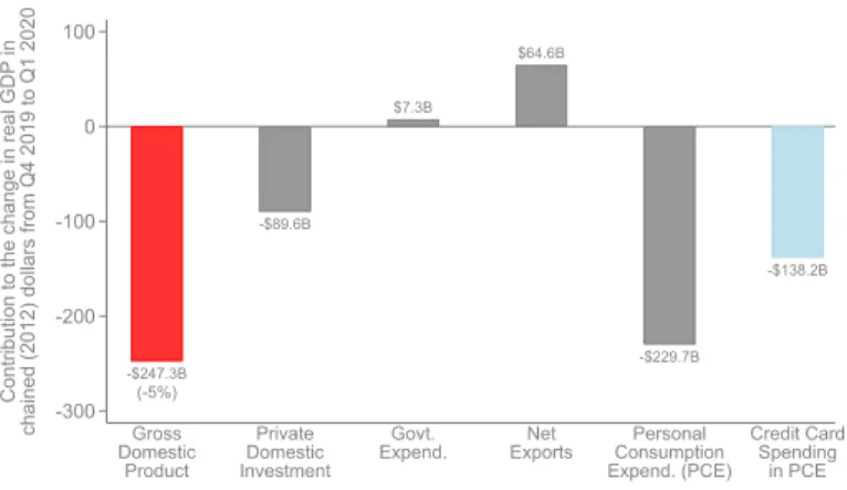
To structure our analysis, we begin from national accounts data released by the Bureau of Economic Analysis (2020). GDP fell by $247 billion (an annualized rate of 5%) from the fourth quarter of 2019 to the first quarter of 2020, shown by the first bar in Figure 1a. GDP fell primarily because of a reduction in personal consumption expenditures (consumer spending), which fell by

$230 billion.¹⁴ Government purchases did not change significantly, while net exports increased by $65 billion and private investment fell by $90 billion.¹⁵ We therefore begin our analysis by studying the determinants of this sharp reduction in consumer spending. We then turn to examine downstream impacts of the reduction in consumer spending on business activity and the labor market.

III.A Consumer Spending

We analyze consumer spending using data on aggregate credit and debit card spending. National accounts data show that spending that is well captured on credit and debit cards – essentially all spending excluding housing, healthcare, and motor vehicles – fell by approximately $138 billion, comprising roughly 60% of the total reduction in personal consumption expenditures.¹⁶

Benchmarking. We begin by assessing whether the credit card data track patterns in corresponding spending categories in the national accounts. Figure 1b plots spending on retail services (excluding auto-related expenses) in the Affinity Solutions credit card data alongside the Monthly

14. GDP is released at a quarterly level in the U.S. The reduction in consumer spending occurred in the last two weeks of March (Figure 2 below); hence the first quarter GDP estimates capture about one-sixth of the reduction in spending due to the COVID shock.

15. Most of the reduction in private investment was driven by a reduction in inventories and equipment investment in the transportation sector, both of which are plausibly a response to reductions in current and anticipated consumer spending. The increase in net exports was driven primarily by a reduction in imports, with a large reduction in imports of travel and transporation services in particular, again reflecting a change in domestic consumer spending behavior.

16. The rest of the reduction is largely accounted for by healthcare and motor vehicle expenditures; housing expenditures did not change significantly. We view the incorporation of data sources to study these other major components of spending as an important direction for future work; however, we believe that the mechanisms discussed below may apply at least qualitatively to those sectors as well.

(17)

Retail Trade Survey (MRTS), one of the main inputs used to construct the national accounts. Both series are indexed to have a value of 1 in January 2020; each point shows the level of spending in a given month divided by spending in January 2020. Figure 1c replicates Figure 1b for spending on food services. In both cases, the credit/debit card spending series closely tracks the inputs that make up the national accounts. In particular, both series show a rapid drop in food services spending in March and April 2020 and a smaller drop in retail spending, along with a recent increase in May. Given that credit card spending data closely tracks the MRTS at the national level, we proceed to use it to disaggregate the national series in several ways to understand why consumer spending fell so sharply.

Heterogeneity by Income. We begin by examining spending changes by household income. We do not directly observe cardholders’ incomes in our data; instead, we proxy for cardholders’ incomes using the median household income in the ZIP code in which they live (based on data from the 2014- 18 American Community Survey). ZIP-codes are strong predictors of income because of the degree of segregation in most American cities; however, they are not a perfect proxy for income and can be prone to bias in certain applications, particularly when studying tail outcomes (Chetty et al. 2020).

To evaluate the accuracy of our ZIP code imputation procedure, we compare our estimates to those of Farrell et al. (2020), who observe cardholder income directly based on checking account data for clients of JPMorgan Chase. Our estimates are closely aligned with those estimates, suggesting that the ZIP code proxy is reasonably accurate in this application.¹⁷

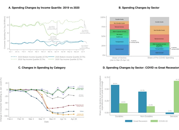
Figure 2a plots a seven-day moving average of total daily card spending for households in the bottom vs. top quartile of ZIP codes based on median household income.¹⁸ The solid line shows data from January to May 2020, while the dashed line shows data for the same days in 2019 as a reference. Spending fell sharply on March 15, when the National Emergency was declared and the threat of COVID became widely discussed in the United States. Spending fell from $7.9 billion per day in February to $5.4 billion per day by the end of March (a 31% reduction) for high-income households; the corresponding change for low-income households was $3.5 billion to $2.7 billion (a 23% reduction). Because high-income households both cut spending more in percentage terms

17. Farrell et al. (2020) report an eight percentage point (pp) larger decline in spending for the highest income quartile relative to the lowest income quartile in the second week of April. Our estimate of the gap is also eight pp at that point, although the levels of the declines in our data are slightly smaller in magnitude for both groups. The JPMorgan Chase data cannot themselves be used for the analysis that follows because there are no publicly available aggregated series based on those data at present.

18. We estimate total card spending by multiplying the raw totals in the Affinity Solutions data by the ratio of total spending on the categories shown in the last bar of Figure 1a in PCE to total spending in the Affinity data in January 2020.

(18)

and accounted for a larger share of aggregate spending to begin with, they account for a much larger share of the decline in total spending in the U.S. than low-income households. We estimate that as of mid-April, top-quartile households accounted for 39% of the aggregate spending decline after the COVID shock, while bottom-quartile households accounted for only 13% of the decline.

This gap grew even larger after stimulus payments began in mid-April. By mid June, top-quartile households accounted for over half of the total spending decline in the U.S. and were still spending 15% less than their January levels, whereas bottom-quartile households were spending almost the same amount they were in 2019. This heterogeneity in spending changes by income is much larger than that observed in previous recessions (Petev, Pistaferri, and Eksten 2011, Figure 6) and plays a central role in understanding the downstream impacts of COVID on businesses and the labor market, as we show below.

Heterogeneity Across Sectors. Next, we disaggregate the change in total spending across categories to understand why households cut spending so rapidly. In particular, we seek to distinguish two channels: reductions in spending due to loss of income vs. fears of contracting COVID.

The left bar in Figure 2b plots the share of the total decline in spending from the pre-COVID period to mid-April accounted for by various categories. Nearly three-fourths of the reduction in spending comes from reduced spending on goods or services that require in-person contact (and thereby carry a risk of COVID infection), such as hotels, transportation, and food services.¹⁹ This is particularly striking given that these goods accounted for only one-third of total spending in January, as shown by the right bar in Figure 2b.

Next, we zoom in to specific subcategories of spending that differ sharply in the degree to which they require physical interaction in Figure 2c. Spending on luxury goods such as installation of home pools and landscaping services – which do not require in-person contact – increased slightly after the COVID shock; by contrast, spending on restaurants, beauty shops, and airlines all plummeted sharply. Consistent with these substitution patterns, spending at online retailers increase sharply:

online purchases comprised 11% of retail sales in 2019 vs. 22% in April and May of 2020 (Mastercard 2020).²⁰ A conventional reduction in income or wealth would typically reduce spending on all goods as predicted by their Engel curves (income elasticities); the fact that the spending reductions vary so sharply across goods that differ in terms of their health risks lends further support to the hypothesis that it is health concerns rather than a lack of purchasing power that drove spending reductions.

19. The relative shares of spending reductions across categories are similar for low- and high-income households (Appendix Figure 4); what differs is the level of spending reduction, as discussed above.

20. We are unable to distinguish online and in-store transactions in the Affinity Solutions data.

(19)

These patterns of spending reductions are particularly remarkable when contrasted with those observed in prior recessions. Figure 2d compares the change in spending across categories in national accounts data in the COVID recession and the Great Recession in 2009-10. In the Great Recession, nearly all of the reduction in consumer spending came from a reduction in spending on goods; spending on services was almost unchanged. In the COVID recession, 67% of the reduction in total spending came from a reduction in spending on services, as anticipated by Mathy (2020).

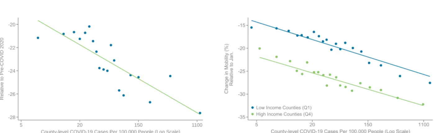
Heterogeneity by COVID Incidence. To further evaluate the role of health concerns, we next turn to directly examine the association between incidence of COVID across areas and changes in spending. Figure 3a presents a binned scatterplot of changes in spending from January to April vs. the rate of detected COVID cases by county. To construct this figure, we divide the x variable (COVID cases) into 20 bins, each of which contain 5% of the population, and plot the mean value of the x and y variables within each bin. Areas with higher rates of COVID infection experience significantly larger declines in spending, a relationship that holds conditional on controls for median household income and state fixed effects (Appendix Figure 5).²¹

To examine the mechanism driving these spending reductions more directly, in Figure 3b, we present a binned scatterplot of the amount of time spent outside home (using anonymized cell phone data from Google) vs. COVID case rates, separately for low- and high-income counties (median household income in the bottom vs. top income quartile). In both sets of areas, there is a strong negative relationship: people spend considerably less time outside home in areas with higher rates of COVID infection. The reduction in spending on services that require physical, in- person interaction (e.g., restaurants) is mechanically related to this simple but important change in behavior.

At all levels of COVID infection, higher-income households spend less time outside. Figure 3c establishes this point more directly by showing that time spent outside home falls monotonically with household income across the distribution. These results help explain why the rich reduce spending more, especially on goods that require in-person interaction: high-income people appar- ently self-isolate more, perhaps by working remotely or because they have larger living spaces.

In sum, disaggregated data on consumer spending reveals that spending in the initial stages of the pandemic fell primarily because of health concerns rather than a loss of current or expected income. Indeed, income losses were relatively modest because relatively few high-income individuals

21. Note that there is a substantial reduction in spending even in areas without high rates of realized COVID infection, which is consistent with widespread concern about the disease even in areas where outbreaks did not actually occur at high rates.

(20)

lost their jobs (Cajner et al. 2020) and lower-income households who experienced job loss had their incomes more than replaced by unemployment benefits (Ganong, Noel, and Vavra 2020). As a result, national accounts data actually show an increase in total income of 13% from March to April 2020. This result implies that the central channel emphasized in Keynesian models that have guided policy responses to prior recessions – a fall in aggregate demand due to a lack of purchasing power – has been less important in the early stages of the pandemic, partly as a result of policies such as increases in unemployment benefits that offset lost earnings. Rather, the key driver of residual changes in aggregate spending is a contraction in firms’ ability to supply certain goods, namely services that carry no health risks. We now show that this novel source of spending reductions leads to a distinct pattern of downstream impacts on businesses and the labor market, potentially calling for different policy responses than in prior recessions.

III.B Business Revenues

We now turn to examine how reductions in consumer spending affect business activity. Conceptu- ally, we seek to understand how a change in revenue for a given firm affects its decisions: whether to remain open, how many employees to retain, what wage rates to pay them, how many new people to hire. Ideally, one would analyze these impacts at the firm level, examining how the customer base of a given firm affected its revenues and employment decisions. Lacking firm-level data, we use geographic variation as an instrument for the spending shocks that firms face. The motivation for this geographical approach is that spending fell primarily among high-income households in sectors that require in-person interaction, such as restaurants. Most of these goods are non-tradable products produced by small local businesses who serve customers in their local area.²² We therefore use differences in average incomes and rents across ZIP codes as a source of variation in the magnitude of the spending shock that small businesses face.²³

Benchmarking. We measure small business revenues using data from Womply, which records revenues from credit card transactions for small businesses (as defined by the Small Business Ad- ministration). Business revenues in Womply closely track patterns in the Affinity total spending

22. 56% of workers in food and accommodation services and retail (two major non-tradeable sectors) work in establishments with fewer than 50 employees.

23. We focus on small businesses because their customers are typically located near the business itself; larger businesses’ customers (e.g., large retail chains) are more dispersed, making the geographic location of the business less relevant. One could also in principle use other groups (e.g., sectors) instead of geography as instruments. We focus primarily on geographic variation because the granularity of the data by ZIP code yields much sharper variation than what is available across sectors and arguably yields comparisons across more similar firms (e.g., restaurants in different neighborhoods rather than airlines vs. manufacturing).

(21)

data, especially in sectors with a large share of small businesses, such as food and accommodation services (Appendix Figure 6).²⁴

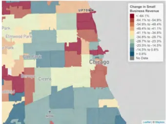
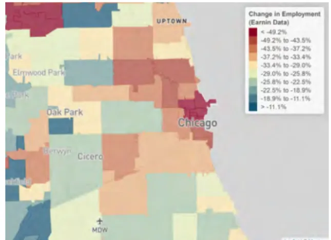
Heterogeneity Across Areas. We begin our analysis of the Womply data by examining how small business revenues changed in low- vs. high-income ZIP codes from a baseline period prior the COVID shock (January 5 to March 7, 2020) to the weeks immediately after the COVID shock before the stimulus program began (March 22 to April 20, 2020). Figure 4 maps the change in small business revenue by ZIP code in three large metro areas: New York City, San Francisco, and Chicago. There is substantial heterogeneity in revenue declines across areas. For example, average revenue declines range from -87% (or below) in the lowest-income-decile of ZIP codes to -12% (or above) in the top-income-decile in New York City.²⁵

In all three cities, revenue losses are largest in the most affluent parts of the city. For example, small business lost 73% of their revenue in the Upper East Side in New York, compared with 14%

in the East Bronx; 67% in Lincoln Park vs. 38% in Bronzeville on the South Side of Chicago; and 88% in Nob Hill vs. 37% in Bayview in San Francisco. Revenue losses are also large in the central business districts in each city (lower Manhattan, the Loop in Chicago, the Financial District in San Francisco), likely a direct consequence of the fact that many workers who used to work in these areas are now working remotely. But even within predominantly residential areas, businesses located in more affluent neighborhoods suffered much larger revenue losses, consistent with the heterogeneity in spending reductions observed in the Affinity data.²⁶ More broadly, cities that have experienced the largest declines in small business revenue on average tend to be affluent cities – such as New York, San Francisco, and Boston (Table 1).

Figure 5a generalizes these examples by presenting a binned scatter plot of percent changes in small business revenue vs. median household incomes, by ZIP code across the entire country.²⁷ We observe much larger reductions in revenue at local small businesses in affluent ZIP codes. In the richest 5% of ZIP codes, small business revenues fell by 60%, as compared with 40% in the poorest 5% of ZIP codes.²⁸

24. In sectors that have a bigger share of large businesses – such as retail – the Womply small business series exhibits a larger decline during the COVID crisis than Affinity (or MRTS). This pattern is precisely as expected given other evidence that consumers shifted spending toward large online retailers such as Amazon (Alexander and Karger 2020).

25. Very little of this variation is due to sampling error: the reliability of these estimates across ZIP codes within counties exceeds 0.8, i.e., more than 80% of the variance within each of these maps is due to signal rather than noise.

26. We find a similar pattern when controlling for differences in industry mix across areas; for instance, the maps look very similar when we focus solely on small businesses in food and accommodation services (Appendix Figure 7).

27. Appendix Figure 8 also provides a national map of the changes in small business revenue.

28. Of course, households do not restrict their spending solely to businesses in their own ZIP code. An alternative way to establish this result at a broader geography is to relate small business revenue changes to the degree of income inequality across counties. Counties with higher Gini coefficients experienced large losses of small business revenue

(22)

As discussed above, spending fell most sharply not just in high-income areas, but particularly in high-income areas with a high rate of COVID infection. Data on COVID case rates are not available at the ZIP code level; however, one well established predictor of the rate of spread of COVID is population density: the infection spreads more rapidly in dense areas. Figure 5b shows that small business revenues fell more heavily in more densely populated ZIP codes.²⁹

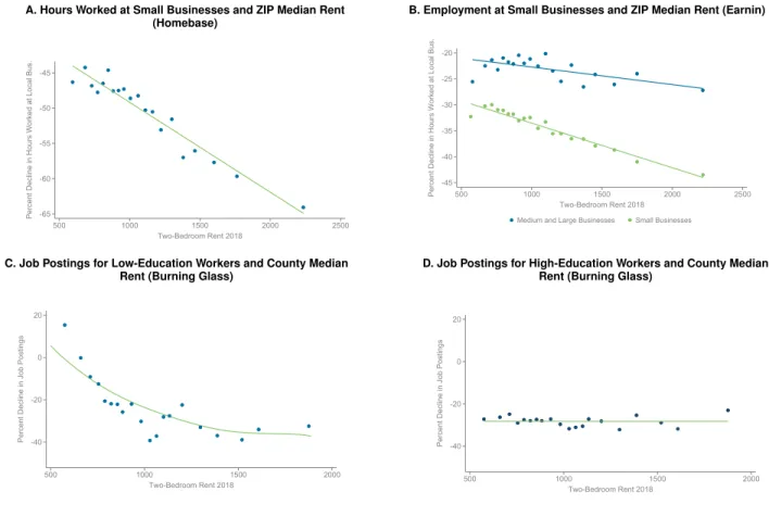
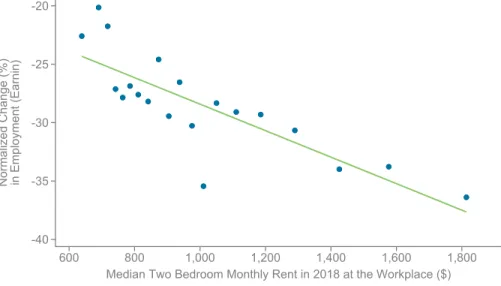
Figure 5c combines the income and population density mechanisms by plotting revenue changes vs. median rents (for a two bedroom apartment) by ZIP code. Rents are a simple measure of the affluence of an area that combine income and population density: the highest rent ZIP codes tend to be high-income, dense areas such as Manhattan. Figure 5c shows a particularly steep gradient of revenue changes with respect to rents: revenues fell by less than 30% in the lowest-rent ZIP codes, compared with more than 60% in the highest-rent ZIP codes. This relationship is essentially unchanged when controlling for worker density in the ZIP code and county fixed effects (Appendix Table 3).

In Figure 5d, we examine heterogeneity in this relationship across sectors that require different levels of physical interaction: food and accommodation services and retail trade (which largely require in-person interaction) vs. finance and professional services (which largely can be conducted remotely). Revenues fall much more sharply for food and retail in higher-rent areas; in contrast, there is essentially no relationship between rents and revenue changes for finance and professional services. These findings show that businesses that cater in person to the rich are those that lost the most businesses. Naturally, many of those businesses are located in high-income areas given people’s preference for geographic proximity in consuming services.

As a result of this sharp loss in revenues, small businesses in high-rent areas are much more likely to close entirely. We measure closure in the Womply data as reporting zero credit card revenue for three days in a row. Appendix Figure 10 shows that 55% of small businesses in the highest-rent ZIP codes closed, compared with 40% in the lowest rent ZIP codes. The extensive margin of business closure accounts for most of the decline in total revenues.

Because businesses located in high-rent areas lose more revenue in percentage terms and tend to account for a greater share of total revenue to begin with, they account for a very large share of

(Appendix Figure 9a). This is particularly the case among counties with a large top 1% income share (Appendix Figure 9b). Poverty rates are not strongly associated with revenue losses at the county level (Appendix Figure 9c), showing that it is the presence of the rich in particular (as opposed to the middle class) that is most predictive of economic impacts on local businesses.

29. Consistent with this pattern, total spending levels and time spent outside also fell much more in high population density areas.

(23)

the total loss in small business revenue. More than half of the total loss in small business revenues comes from business located in the top-quartile of ZIP codes by rent; only 8% of the revenue loss comes from businesses located in the bottom quartile. We now examine how the incidence of this shock is passed on to their employees.

III.C Impacts on Employment Rates and Low-Income Workers

We analyze the impacts of the COVID shock on employment using data from two sources: Earnin, which provides data on hours, wages, and employment rates for low-wage (bottom quintile) workers across a broad range of industries and Homebase, which provides analogous data for hourly workers in small businesses, especially restaurants and retail shops.

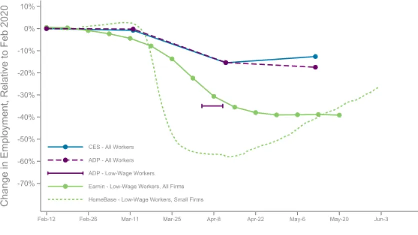
Benchmarking. As with the other series analyzed above, we begin by benchmarking changes in these series to nationally representative benchmarks. Figure 6a plots employment rates from the nationally representative Current Employment Statistics for all workers alongside the overall Earnin series and Homebase series. We also include theNational Employment Report from ADP, a large payroll processor that covers nearly 20% of employment in the U.S. The ADP data are reweighted to provide estimates that are intended to represent all workers in the U.S. Cajner et al. (2020) use ADP data to report estimates of the decline in employment by worker wage quintile, showing that employment rates fell much more sharply for lower-wage workers. We plot the estimate they report for workers in the bottom quintile as of April 11 in Figure 6a. Consistent with the findings of Cajner et al. (2020), the CES and ADP overall worker series exhibit smaller declines in employment rates than the series that focus on low-wage workers. The ADP estimate for low-wage workers is roughly aligned with decline observed in Earnin. Homebase exhibits a much larger decline than Earnin.

The differences between these series are largely explained by differences in industry and size composition. Figure 6b establishes this result by replicating Figure 6a for workers in Accom- modation and Food Services, for which the Earnin series and ADP series are closely aligned.³⁰ Furthermore, when we restrict Earnin to small firms – with less than 50 employees, comparable to the typical sizes of firms in the Homebase data – we find alignment between the Earnin and Homebase samples as well. Based on this benchmarking exercise, we conclude that Earnin provides a good representation of employment rates for low-wage workers across sectors, while Homebase provides estimates that are representative of workers at small businesses, particularly in restaurants

30. Since estimates for Accommodation and Food Services are unavailable in ADP’s National Employment Report, we use their Leisure and Hospitality Series.