The name of the double precision spec version begins with a "D_." The single precision-specific version begins with an "S_". However, legacy code that calls routines in the previous version of the library without using a "using" statement will continue to work as before.
Programming Tips
IMSL STAT/LIBRARY Introduction · xv Users wishing to update existing programs to call new generic versions of the routines must modify their calls to the existing routines to match the new calling sequences and use routine-specific interface modules or an all-encompassing module “imsl_libraries”.
Optional Subprogram Arguments
Error Handling
Printing Results
Missing Values
Routines that Accumulate Results over Several Calls
Using IMSL Fortran Library on Shared-Memory Multiprocessors
Basic Statistics
Routines
Frequency Tabulations
Usage Notes
Frequency Tabulations
Other analyzes of discrete or count data can be performed using the IMSL routines in Chapter 5, "Categorical and Discrete Data Analysis."
Univariate Summary Statistics
Ranks and Order Statistics
Parametric Estimates and Tests
Grouped Data
Continuous Data in a Table
2 · Chapter 1: Basic Statistics IMSL STAT/LIBRARY frequency tables fundamentally assume that the data are discrete and count the number of observations with each value.
OWFRQ
This option may be appropriate if we do not know the range of the data. Note that the midpoints of the class intervals, output in the DIV, are not "pretty" numbers.
TWFRQ
For example, "4" in the second row and second column of the output is the first number representing a frequency. The midpoints of the intervals for the first variable are output in DIVX and for the second in DIVY.
FREQ
IMSL STAT/LIBRARY Chapter 1: Basic Statistics · 15 MAXCL — An upper bound for the sum of the number of distinct values represented by all the. TABLE — Vector of length NCLVAL(1) *NCLVAL(2) * ¼ *NCLVAL(NCLVAR) containing the frequencies in the cells of the table to be matched.
UVSTA
LDX — Leading dimension of X exactly as specified in the dimension declaration in the calling program. A weight of zero results in the row being counted and updates are made to statistics and the number of missing values.
RANKS
For this option, the output values in SCORE are the expected values of the normal order statistic from a sample size of NOBS. For this option, the output values in SCORE are the expected values of the exponential order statistic from a sample size of NOBS.
LETTR
The routine LETTR calculates the median ("M"), the minimum, the maximum, and other depths or "letter values" - hinges ("H"), eighths ("E"), sixteenths ("D"), etc. —as specified by NUM. Examples and discussion of the use of letter values are given by Tukey (1977, Chapter 2) and by Velleman and Hoaglin (1981, Chapter 2).
ORDST
In the first example, the first five order statistics are obtained from a sample of size 30. In the second example, the last five order statistics are obtained from a sample of size 30.
EQTIL
Any IOS value must be greater than 0. and less than or equal to the number of valid observations. The EQTIL routine determines the empirical quantiles, as shown in the QPROP vector, from the data in X.
TWOMV
22 Lower confidence limit for the ratio between the variance of the first population and the second. 23 Upper confidence limit for the ratio between the variance of the first population and the second.
BINES
The BINES routine calculates the point estimate and confidence interval for the parameter p of the binomial distribution using the number of "hits" K in a sample of size N from the binomial distribution with a probability function. The BETIN routine is used to evaluate the critical values (see Chapter 17, Probability Distribution Function and Inverses).
POIES
Since the binomial is a discrete distribution, it is not possible to construct an exact CONPER% confidence interval for all values of CONPER. The routine POIES calculates a point estimate and a confidence interval for the parameter q of a Poisson distribution.
NRCES
For more than one observation, the estimates are obtained as above and then divided by the number of observations, NOBS. Estimate of mean: 4.4990 Estimate of standard deviation: 1.2304 Estimate of variance of mean estimate: 0.0819 Estimate of variance of variance estimate: -0.0494 Estimate of covariance of mean and variance: -0.0019 Number of exact observations right: 12 or 12 : 3 Number of left-censored observations: 2 Number of interval-censored observations: 1.
GRPES
The standard deviation (STAT(3)), on the other hand, is calculated by using the sum of the frequencies minus one as the divisor. If any of the class scores are negative, the geometric and harmonic means are not calculated, and NaN (not a number) is stored as the value of STAT(11).
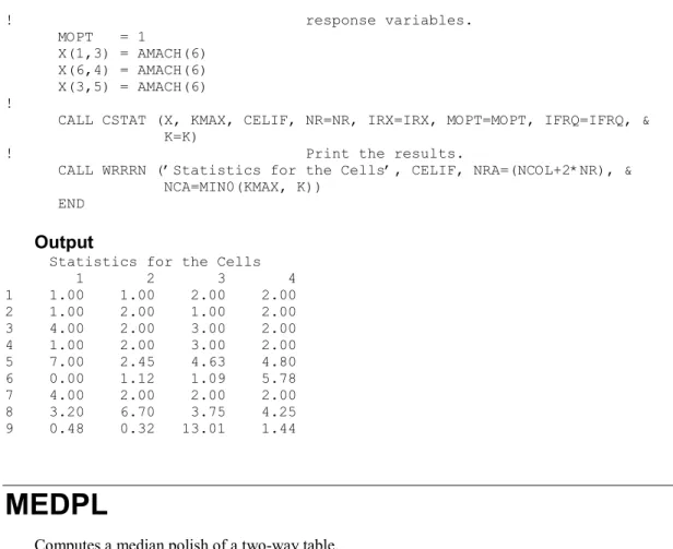
CSTAT
Each combination of values of the classification variables is stored in the first m rows of CELIF. The frequency variable indicates that the values of the classification and response variables in the first.
MEDPL
Regression
Routine
Simple Linear Regression
OPOLY 292 Centering of variables and generation of cross products..GCSCP 296 Transformation of coefficients for a second order model.
Simple Linear Regression
Multiple Linear Regression
Variable selection can be performed by RBEST (page 231), which performs all best subset regressions, or by RSTEP (page 237), which performs stepwise regression. The routines GSWEP and RSUBM can be invoked before RBEST to force certain variables into all the models considered by RBEST.
Polynomial Model
However, the computer time and memory requirements for RBEST can be much higher than for RSTEP if the number of candidate variables is large. The RSUBM routine can be called after GSWEP or RSTEP to extract the symmetric submatrix whose rows and columns have been swept, ie. which rows and columns entered the stepwise model.
Multivariate General Linear Model
Column 2 Column 3 Column 4
The routines in this chapter are designed to handle linear dependence of the regressors, ie. The n ´p matrix X (the matrix of regressors) in the general linear model may have rank less than p. In the case of non-full rank, not all linear combinations of the regression coefficients can be estimated.
Nonlinear Regression Model
The sum of squares and matrix cross product error (SCPE) output from model fitting is required to enter the RHPTE. Additionally, the hypothesized sum of squares and cross product matrix (SCPH), which can be calculated using RHPSS, is required to enter RHPTE.
Weighted Least Squares
The RHPSS routine (page 176) computes the matrix of sums of squares and cross products for the general linear hypothesis H B U = G for the multivariate general linear model Y = XB + e with possible linear equality constraints AB = Z. The RHPTE routine (page 183) computes several test statistics and approximate p-values for the multivariate general linear hypothesis.
Summary Statistics
80 · Chapter 2: Regression IMSL STAT/LIBRARY the frequencies are entered in column IFRQ of the data matrix. In the case where no intercept is indicated (INTCEP=0), the total sum of squares is the sum of the squares of yi – the so-called corrected total sum of squares, which is denoted by.
Tests for Lack of Fit
SQSS — A two-dimensional matrix containing the sequential sums of squares as one column and the associated statistics (including degrees of freedom, F statistic, and p-value) in the remaining columns.
Diagnostics for Individual Cases
The residual mean square for the regression in which the i-th case is dropped is Cook's distance for the i-th case is a measure of how much an individual case affects the estimated regression coefficients.
Transformations
When the responses are non-normal and their distribution is known, a transformation of the responses can often be selected so that the transformed responses closely match the assumptions of the regression model. If the distribution of responses is not known, the data can be used to select a transformation so that the transformed responses can better fit the regression model.
Alternatives to Least Squares
Predicted values and confidence intervals for combinations of independent variable settings that are not used in the regression fit calculation are often desired. These additional lines must contain the desired independent variable settings along with responses that equal NaN.
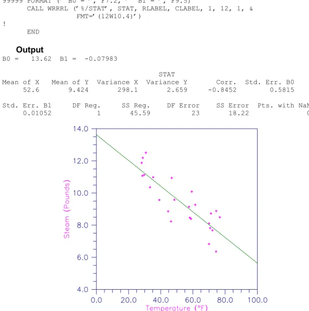
RLINE
In fitting regression models, any row of the data matrix containing NaNs for the independent, dependent, weight, or frequency variables is omitted from the computation of the regression parameters. NaN cases will not be used in determining the regression parameter estimates, and a predicted value and confidence interval will be calculated from the given settings of the independent variables.
RONE
13 Estimated standard deviation of the model error 14 Mean of response (dependent) variable 15 Coefficient of variation (in percent). TESTLF — Vector of length 10 containing statistics regarding the model's lack of fit test.
RINCF
If INTCEP = 1, SSX is the sum of the squares of deviations of the independent variable from its mean. SWTFY0 — S2/SWTFY0 is the estimated variance of the future response (or future response mean) to be controlled.
RINPF
When the variance of the ei's are all equal, ordinary least squares must be used, this corresponds to all wi = 1. The wi's are the weights to be used in the fitting of the model.
RLSE
In the case INTCEP = 1, the total sum of squares is the sum of the squares of the deviations of yi from the mean. After completing the final calculations, if the ith regressor is declared linear.
RCOV
LDB — Front dimension of B exactly as specified in the dimension statement in the calling program. LDR — Front dimension of R exactly as specified in the dimension statement in the calling program.
RGIVN
XMIN — Vector of length INTCEP + |IIND| which contains the minimum values for each of the regressors. XMAX — Vector of length INTCEP + |IIND| which contains the maximum values for each of the regressors.
RGLM
CLVAL — A vector of length NCLVAL(1) + NCLVAL(2) + ¼ + NCLVAL(NCLVAR) containing the values of the classification variables. This means that the intercept estimate and the R matrix are for uncentered data.
RLEQU
LDH — The leading dimension of H exactly as specified in the calling program's dimension statement. A positive diagonal element means that the row/column corresponds to the data for the regressors in the reduced model.
RSTAT
156 · Chapter 2: Regression IMSL STAT/LIBRARY LDSQSS — Front dimension of SQSS exactly as specified in the dimension statement in . If an intercept is in the model, the regression sum of squares is adjusted for the mean, i.e.
RCOVB
The RCOVB routine computes an estimated variance-covariance matrix of the regression parameters estimated from the R matrix in several models. RCOVB is then used to calculate the estimated asymptotic variance-covariance matrix of the estimated nonlinear regression parameters.
CESTI
LDHP - Main HP dimension exactly as specified in the calling program's dimension statement. A sum of squares can then be calculated for the fully testable hypothesis (see routine RHPSS).
RHPSS
Form VTV, which is the required matrix of sum of squares and cross products output in SCPH. The sum of squares and cross products matrix is calculated for the third independent variable in the model.
RHPTE
The sum of squares and cross products matrix is calculated for the third independent variable in the model using RHPSS (page 176). Routine RHPTE is used to test whether the third independent variable should be included in the regression.