We discuss cross-sectional and time-series regression data, least squares, and maximum likelihood model fitting. The explicit time series modeling approach to forecasting that we have chosen to highlight is the autoregressive integrated moving average (ARIMA) model approach.
CHAPTER
Introduction to Forecasting
- THE NATURE AND USES OF FORECASTS
- SOME EXAMPLES OF TIME SERIES
- RESOURCES FOR FORECASTING
- CHAPTER 2
Other important characteristics of the forecasting problem are the forecast horizon and the forecast interval. Data analysis is an important preliminary step for choosing the forecasting model to be used.

Statistics Background for Forecasting
INTRODUCTION
The reason for this careful distinction between forecast errors and residuals is that models usually fit historical data better than they predict. That is, the residuals from a model fitting process will almost always be smaller than the forecast errors experienced when that model is used to predict future observations.
GRAPHICAL DISPLAYS .1 Time Series Plots
The forecast error resulting from a forecast of y1 made in the period t - r is the lead - T.
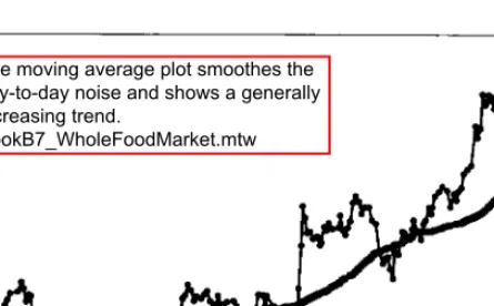
Plotting Smoothed Data
A time series chart of Whole Foods Market stock price with a 50-day moving average is shown in Figure 2-6. The plot of the moving average softens the daily noise and generally shows an upward trend.

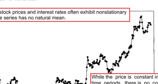
NUMERICAL DESCRIPTION OF TIME SERIES DATA .1 Stationary Time Series
- Autocovariance and Autocorrelation Functions
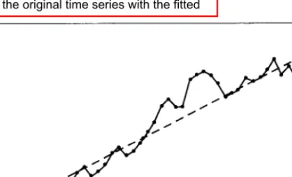
The chemical process viscosity readings shown in Figure 1.11 are an example of a time series that benefits from smoothing to estimate models. The time series data of pharmaceutical product sales and chemical viscosity readings, originally shown in Figures 1.2 and 1.3, are examples of stationary time series.
USE OF DATA TRANSFORMATIONS AND ADJUSTMENTS .1 Transformations
- Trend and Seasonal Adjustments
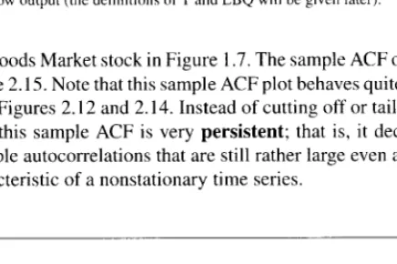
The trend analysis chart in Figure 2.17 shows the original time series with the fit line. Results of a Mini-tab time series analysis of the beverage shipments are in Figure 2.23, which shows the original data (labeled "Actual") along with the fitted trend line ("Trend") and the predicted values ("Fit") of the additive model with both the trend and seasonal components.
GENERAL APPROACH TO TIME SERIES MODELING AND FORECASTING
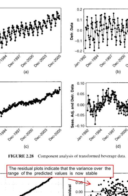
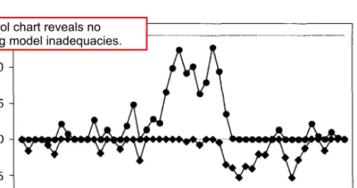
The results from the decomposition analysis of the natural log transformed beverage shipment data are shown in Figure 2.27, with the transformed data, the fitted trend line. The remaining plots in Figure 2.29 show that the variance over the range of predicted values is now stable (Figure 2.29b), and there are no problems with the assumption of normality (Figures 2.29a,c).
EVALUATING AND MONITORING FORECASTING MODEL PERFORMANCE
- Forecasting Model Evaluation
- Choosing Between Competing Models
- Monitoring a Forecasting Model
Because the MSE estimates the variance of the forecast errors one step ahead, we have The normal probability plot of the one-step-ahead forecast errors from Table 2.3 is shown in Figure 2.32. The estimate of the standard deviation of the one-step-ahead forecast errors is based on the average of the moving ranges.
This standard deviation estimate would be used to construct the control limits on the control chart for prediction errors. Note that both an individual control chart of the one-step-ahead prediction errors and a control chart of the moving ranges of these prediction errors are provided. All prediction errors that are one step ahead are plotted within their control limits (and the moving range is also plotted within their control limits).

Take the first difference in the natural logarithm of the data and plot this new time series. Now plot the first difference in the time series and calculate the sample autocorrelation function for the first differences. Now plot the first difference in the GDP time series and calculate the sample autocorrelation function for the first differences.
What is the variance of this lead-one forecast error') .. 2.28 Suppose that a simple moving average of span N is used to forecast a time series that varies randomly about a constant. it is.
CHAPTER 3
Regression Analysis and Forecasting
INTRODUCTION
The regression models in Eq. 3.1) and (3.2) are linear regression models because they are linear in the unknown parameters (/)'s) and not because they necessarily describe linear relationships between the response and the regressors. is a linear regression model because it is linear in the unknown parameters and {32, although it describes a quadratic relationship between ·'· and x. Regression models such as Eq. 3.3) can be used to remove seasonal effects from time series data (see Section 2.4.4 where models like this were introduced). The regression model for cross-sectional data is written as .. where the subscript i is used to denote each individual observation lor case) in the data set and n represents the number of observations.
LEAST QUANTUM ESTIMATION IN LINEAR REGRESSION MODELS 75 and the regressors are time series, so the regression model involves time series data. The regression model for time series data is written as. 3.4), note that we have changed the observation or case subscript from i to t to emphasize that the response and the predictor variables are time series. This is an important application of regression models in forecasting, but not the only one.
LEAST SQUARES ESTIMATION IN LINEAR REGRESSION MODELS
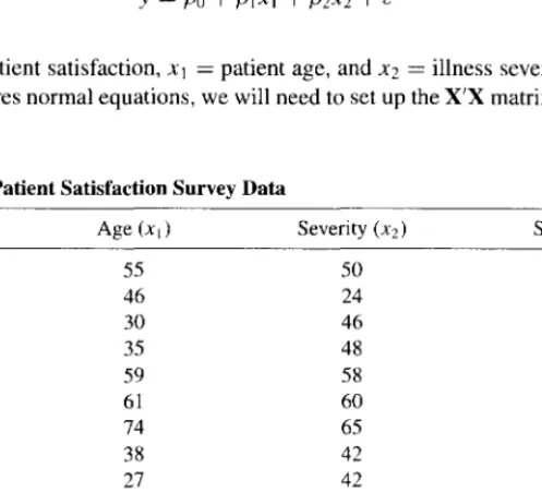
The solutions of the normal equations will be the least squares estimators of the regression coefficients of the model. If the model is correct (it has the correct form and includes all relevant predictors), the least squares estimator ~ is an unbiased estimator of the model parameters f3; this is. To solve normal least squares equations, we will need to set the X'X and X'y matrix.
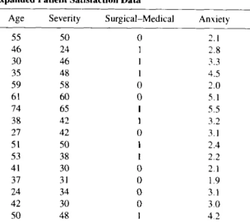
LEAST SQUARES ESTIMATION IN LINEAR REGRESSION MODELS 81 Using Eq. 3.13), we can find the least squares estimates of the parameters in the regression model as where x 1 = the patient's age and x2 = the severity of the disease, and we have reported the regress-. sion coefficients to three decimal places. TABLE 3.3 Minitab regression output for the patient satisfaction data in Table 3.2 (Continued). Because there are only two parameters, it is easy to solve the normal equations directly, resulting in least squares estimators.
STATISTICAL INFERENCE IN LINEAR REGRESSION
- Test for Significance of Regression
- Confidence Intervals on the Mean Response
The quantities in the numerator and denominator of the test statistic F0 are called mean squares. J depends on all the other regressor variables. 3.27), Ja2C11 , is usually called the standard error of the regression coefficient. To find the contribution of the terms in 131 to the regression, we fit the model, assuming that the null hypothesis.
The calculated value of F0 will be exactly equal to the square of the t-test statistic t0. The reduced model is the model with all the predictors in the vector 131 equal to zero. This decrease in the adjusted R2 is an indication that the additional variables did not contribute to the explanatory power of the model.
PREDICTION OF NEW OBSERVATIONS
The PI formula in Eq. 3.46) is very similar to the formula for the CI on the mean, Eq. The difference is the "I" in the variance of the prediction error below the square root. It is reasonable that the PI should be longer, since the CI is an interval estimate of the mean of the response distribution at a specific point, while the PI is an interval estimate of a single future observation of the response distribution at that point.
There should be more variability associated with an individual observation than with an estimate of the mean, and this is reflected in the extra length of the PI. Now compare the length of CI and PI for this point with the length of CI and PI for the point x1 = patient age = 60 and x2 = severity = 60 from Example 3.4. The intervals are longer for the point in this example because this point with x1 = patient age = 75 and x2 = severity = 60 is farther from the center of the predictor variable data than the point in Example 3.4.
MODEL ADEQUACY CHECKING .1 Residual Plots
- Measures of Leverage and Influence
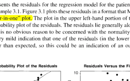
The graph at the top left of the screen is a normal residual probability plot. As hii increases, observation x1 lies farther from the center of the region containing the data. The studentized residuals have unit variance (that is, V(r1) = 1) regardless of the location of the observation x1 when the form of the regression model is correct.
Absolute values of the studentized residuals that are greater than three or four indicate potentially problematic observations. The arrangement of points in the predictor variable space is important in determining many properties of the regression model. As mentioned earlier, H determines the variances and covariances of the predicted response and residuals because.
VARIABLE SELECTION METHODS IN REGRESSION
Note that except for the constant p, D; is the product of the square of the ith student residual and the ratio h;; /(I - h;;. This ratio can be expressed as the distance from the vector x; to the centroid of the remaining data. A variant of the forward selection procedure starts with a model that contains none of the candidate predictor variables and sequentially inserts the variables into the model one by one , until the final equation is produced.
Variables are removed until all predictors remaining in the model have a significant !-statistic. The model with the smallest mean squared error (or its square root, S) is a three-variable model with age, severity, and anxiety. Any of these models is likely to be a good regression model describing the effects of predictor variables on patient satisfaction.
GENERALIZED AND WEIGHTED LEAST SQUARES
- Weighted Least Squares
- Discounted Least Squares
Recall that the covariance matrix of the model parameters in WLS in Eq. Weighted least squares are typically used in situations where the variance of the observations is not constant. Discounted least squares also leads to a relatively simple way to update the estimates of the model parameters after each new observation in the time series.
Since the time origin is shifted to the end of the current time period, forecasting is easy with discounted least squares. The prediction of the observation in the future time period T + r produced at the end of time period T. The updated estimates of the model parameter calculated at the end of time period I are now.
REGRESSION MODELS FOR GENERAL TIME SERIES DATA Many applications of regression in forecasting involve both predictor and response
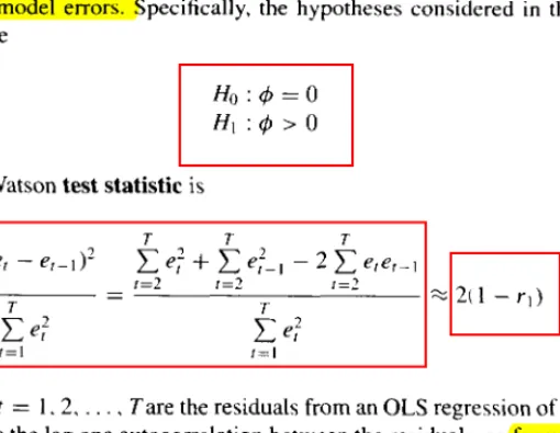
- Detecting Autocorrelation: The Durbin-Watson Test
Suppose that the mean of the model in Eq. with independent and normally distributed errors. Therefore, when the errors are normally and independently distributed, the maximum likelihood estimators of the model parameters {30 and {31 in the linear regression model are identical to the least squares estimators. REGRESSION MODELS FOR GENERAL TIME SERIES DATA 155 where ZaJ2 is the upper a/2 percentage point of the standard normal distribution.
Is the least squares estimator of the slope in the original simple linear regression model unbiased. What is the variance of the slope (/31) for the least squares estimator found in part a. Assume that the variances of the errors are proportional to the time index so that ~t·1.
CHAPTER 4
Exponential Smoothing Methods
- INTRODUCTION
- FIRST-ORDER EXPONENTIAL SMOOTHING
- MODELING TIME SERIES DATA
- SECOND-ORDER EXPONENTIAL SMOOTHING
Visual inspection suggests that a constant model can be used to .. describe the general pattern of the data. As we can see, for the constant process the smoother in Eq. 4.2) is quite effective in providing a clear picture of the underlying pattern. We can therefore expect the variance of the simple exponential smoother to vary between 0 and the variance of the original time series, based on the choice of A.
Note that the choice of initial value has very little effect on the smoothed values over time. Therefore the expected value of the simple exponential smoother for the linear trend model is A method based on adaptive updating of the discount factor, A., after changes in the process is given in section 4.6.4.