Lecture3iDensitymatri

Lecture3iDensitymatri

Recommended reading ^{Nielsen chapter Z 9}

Feymann ^chapter

1.10 The Trace

The trace of an operator is defined as the sum of its diagonal entries:

tr(A)=X

i

hi|A|ii. (1.71)

It turns out that the trace is the same no matter which basis you use. You can see that using completeness: for instance, if|aiis some other basis then

X

i

hi|A|ii=X

i

X

a hi|aiha|A|ii=X

i

X

a ha|A|iihi|ai=X

a ha|A|ai. Thus, we conclude that

tr(A)=X

i

hi|A|ii=X

a

ha|A|ai. (1.72)

The trace is a property of the operator, not of the basis you choose. Since it does not matter which basis you use, let us choose the basis| iiwhich diagonalizes the operator A. Thenh i|A| ii= _iwill be an eigenvalue ofA. Thus, we also see that

tr(A)=X

i

i=sum of all eigenvalues ofA . (1.73)

Perhaps the most useful property of the trace is that it iscyclic:

tr(AB)=tr(BA). (1.74)

I will leave it for you to demonstrate this. Simply insert a convenient completeness relation in the middle ofAB. Using the cyclic property (1.74) you can also move around an arbitrary number of operators, but only in cyclic permutations. For instance:

tr(ABC)=tr(CAB)=tr(BCA). (1.75)

Note how I am moving them around in a specific order: tr(ABC) , tr(BAC). An example that appears often is a trace of the form tr(UAU^†), whereUis unitary operator.

In this case, it follows from the cyclic property that tr(UAU^†)=tr(AU^†U)=tr(A)

Thus, the trace of an operator is invariant by unitary transformations. This is also in line with the fact that the trace is the sum of the eigenvalues and unitaries preserve eigenvalues.

Finally, let| iand| ibe arbitrary kets and let us compute the trace of the outer product| ih |:

tr(| ih |)=X

i

hi| ih |ii=X

i

h |iihi| i 19

Mathematicians ^before

^{start with the physics}

let

^{review the} concept of ^{trace of}

operator

The sum over|iibecomes a 1 due to completeness and we conclude that

tr(| ih |)=h | i. (1.76)

Notice how this follows the same logic as Eq. (1.74), so you can pretend you just used the cyclic property. This formula turns out to be extremely useful, so it is definitely worth remembering.

20

Density ^{Matrices and thermal status}

Let

review

bit ^the Gibbs formalisms

^causielen

system ^described by

Hamiltonian ^{H with} eigenstuff

H Em ^{Im Lm}

If ^this system

equilibrium ^{then the} probability ^{to find}

it in state ^{In will be} given by

In

PEm

2

Moreover

equilibrium ^the expectation ^value of any observable

A ^is given by

A Cml Atm In ³

We

may

^{ask the} following ^{question is there}

^quantum

state 143 ^{which would allow}

^{to write 3}

A

441A 14

^{possible ca}

the ^answer

^For instance

^could naively try

^skate

like in E ^{FI In CST}

But ^then

gives

XIA 143 E ^{Smt Alm Im}

m ^m

which is not ^like

^{It will}

^with

if ^{A happens to be} diagonal

^{the basin Im But} only ^{in that}

The moral of ^the story

^{that it}

^{not possible to attribute}

a

net in ^so

thermal state ^The only ^{exception of}

at

temperature ^{where the system tends to the} ground ^state

In

to attribute

quantum ^{state to the system}

have to generalize ^{the motion of beets The} generalization

called

density ^{matrix which}

usually ^write

^{f the} density ^{matrix of the thermal state is defined}

f fImlm

the expectation ^{value of 4A in}

^{be written using}

the trace

az ^tr C

which ^{in the}

^{tr ga}

Below

try ^{to better motivate why}

^{object such}

6

makes

^But before doing

^let

just ^show you something ^{neat the} decomposition of ^H

ⁱⁿ

^{makes it} convenient ^to study ^{functions of H For instance}

HE f ^{Ent in soul}

H3 _Em EI ^{in Kmt}

and

Thus if ^f

^is

arbitrary ^{function then}

f ^H f ^{f En 1m3cm}

we

just apply ^{f C}

^the eigenvalues ^and multiply ^{by the projectors}

In Kmt

If

^{look at}

that

g.szqe E.PT ^{PFmtmkml Z a}

This ^is

very ^{neat and very} powerful ^way of writhing ^{the thermal} state ^{what is nice about it is that it makes}

^reference

to any

specific ^{basin it} simply ^{writes the state} directly

^function

of ^the Hamiltonian

The partition function

^{be written in}

^{neat way}

z trCEP ^Go

because

EPH ^my

^{PH Im}

^{PEM z}

Thus ^the expectation ^{value 77 may also be written}

as

a7 tIf ^{p C}

Chapter 2

Density matrix theory

2.1 The density matrix

A ket| i is actually not the most general way of defining a quantum state. To motivate this, consider the state|n+iin Eq. (1.47) and the corresponding expectation values computed in Eq. (1.48). This state is always poitingsomewhere: it points at the directionnof the Bloch sphere. It is impossible, for instance, to find a quantum ket which is isotropic. That is, whereh xi=h yi=h zi=0. That sounds strange. The solution to this conundrum lies in the fact that we need to also introduce someclassical uncertaintyto the problem. Kets are only able to encompass quantum uncertainty.

The most general representation of a quantum system is written in terms of an operator ⇢called thedensity operator, ordensity matrix. It is built in such a way that it naturally encompasses both quantum and classical probabilities. But that is not all. We will also learn next chapter that density matrices are intimately related to entanglement. So even if we havenoclassical uncertainties, we will also eventually find the need for dealing with density matrices. For this reason, the density matrix is the most important concept in quantum theory. I am not exaggerating. You started this chapter as a kid. You will finish it as an adult. :)

To motivate the idea, imagine we have a machine which prepares quantum systems in certain states. For instance, this could be an oven producing spin 1/2 particles, or a quantum optics setup producing photons. But suppose that this apparatus is imperfect, so it does not always produces the same state. That is, suppose that it produces a state

| 1iwith a certian probabilityp1or a state| 2iwith a certain probability p2and so on. Notice how we are introducing here aclassical uncertainty. The| iiare quantum states, but we simplydon’t knowwhich states we will get out of the machine. We can have as manyp’s as we want. All we need to assume is that satisfy the properties expected from a probability:

pi2[0,1], and X

i

pi=1 (2.1)

Now letAbe an observable. If the state is | 1i, then the expectation value ofA will beh 1|A| 1i. But if it is| 2ithen it will beh 2|A| 2i. To compute the actual

21

The results ^above

for ^{thermal skates but the idea} of

density ^{matrix is absolutely} general ^{To motivate the reasoning}

behind ^{this I introduce below}

construction of ^the density

matrix ^{which is}

general Hopefully ^{it will} clarify ^{the logic}

behind ^these objects

expectation value ofAwe must therefore perform anaverage of quantum averages:

hAi=X

i

pih i|A| ii (2.2)

We simply weight the possible expectation valuesh i|A| iiby the relative probabilities pithat each one occurs.

What is important to realize is that this type of averagecannotbe writen ash |A| i for some ket| i. If we want to attribute a “state” to our system, then we must generalize the idea of ket. To do that, we use Eq. (1.76) to write

h i|A| ii=tr A| iih i|

Then Eq. (2.2) may be written as hAi=X

i

pitr

A| iih i| =tr⇢ AX

i

pi| iih i| This motivates us to define thedensity matrixas

⇢=X

i

pi| iih i| (2.3)

Then we may finally write Eq. (2.2) as

hAi=tr(A⇢) (2.4)

which, by the way, is the same as tr(⇢A) since the trace is cyclic [Eq. (1.74)].

With this idea, we may now recastallof quantum mechanics in terms of density matrices, instead of kets. If it happens that a density matrix can be written as⇢=| ih |, we say we have apure state. And in this case it is not necessary to use⇢at all. One may simply continue to use| i. For instance, Eq. (2.4) reduces to the usual result:

tr(A⇢)=h |A| i. A state which is not pure is usually called amixed state. In this case kets won’t do us no good and wemustuse⇢.

Examples

Let’ s play with some examples. To start, suppose a machine tries to produce qubits in the state|0i. But it is not very good so it only produces|0iwith probabilityp. And, with probability 1 pit produces the state|1i. The density matrix would then be.

⇢=p|0ih0|+(1 p)|1ih1|= p 0

0 1 p

! .

22

Or it could be such that it produces either|0ior|+i=(|0i+|1i)/p 2. Then,

⇢=p|0ih0|+(1 p)|+ih+|=1 2

1+p 1 p

1 p 1 p

! .

Maybe if our device is not completely terrible, it will produce most of the time|0iand every once in a while, a state| i=cos^✓₂|0i+sin^✓₂|1i, where✓is some small angle.

The density matrix for this system will then be

⇢=p|0ih0|+(1 p)| ih |= p+(1 p) cos²₂^✓ (1 p) sin^✓₂cos₂^✓ (1 p) sin^✓₂cos^✓₂ (1 p) sin²₂^✓

!

Of course, the machine can very well produce more than 2 states. But you get the idea.

Next let’s talk about something really cool (and actually quite deep), called the ambiguity of mixtures. The idea is quite simple: if you mix stu↵, you generally loose information, so you don’t always know where you started at. To see what I mean, consider a state which is a 50-50 mixture of|0iand|1i. The corresponding density matrix will then be

⇢= 1

2|0ih0|+1

2|1ih1|=1 2

1 0 0 1

! .

Alternatively, consider a 50-50 mixture of the states|±iin Eq. (1.11). In this case we get

⇢= 1

2|+ih+|+1

2| ih |=1 2

1 0 0 1

! .

We see that both are identical. Hence, we haveno way to tellif we began with a 50-50 mixture of|0iand|1ior of|+iand| i. By mixing stu↵, we have lost information.

2.2 Properties of the density matrix

The density matrix satisfies a bunch of very special properties. We can figure them out using only the definition (2.3) and recalling thatpi2[0,1] andP

ipi=1 [Eq. (2.1)].

First, the density matrix is a Hermitian operator:

⇢^†=⇢. (2.5)

Second,

tr(⇢)=X

i

pitr(| iih i|)=X

i

pih i| ii=X

i

pi=1. (2.6)

This is thenormalizationcondition of the density matrix. Another way to see this is from Eq. (2.4) by choosingA=1. Then, sinceh1i=1 we again get tr(⇢)=1.

We also see from Eq. (2.8) thath |⇢| iis a sum of quantum probabilities|h | ii|² averaged by classical probabilitiespi. This entails the following interpretation: for an arbitrary state| i,

h |⇢| i=Prob. of finding the system at state| igiven that it’s state is⇢ (2.7)

23

Besides normalization, the other big property of a density matrix is that it ispositive semi-definite, which we write symbolically as⇢ 0. What this means is thatits sandwich in any quantum state is always non-negative. In symbols, if| iis an arbitrary quantum state then

h |⇢| i=X

i

pi|h | ii|² 0. (2.8)

Of course, this makes sense in view of the probabilistic interpretation of Eq. (2.7).

Please note that this doesnot mean that all entries of⇢are non-negative. Some of them may be negative. It does mean, however, that the diagonal entries are always non-negative, no matter which basis you use.

Another equivalent definition of a positive semi-definite operator is one whose eigenvalues are always non-negative. In Eq. (2.3) it already looks as if⇢is in di- agonal form. However, we need to be a bit careful because the| iiare arbitrary states and do not necessarily form a basis (which can be seen explicitly in the examples given above). Thus, in general, the diagonal structure of⇢will be di↵erent. Notwithstanding,

⇢is Hermitian and may therefore be diagonalized by some orthonormal basis| kias

⇢=X

k

k| kih k|, (2.9)

for certain eigenvalues k. Since Eq. (2.8) must be true for any state| iwe may choose, in particular,| i=| ki, which gives

k=h k|⇢|ki 0.

Thus, we see that the statement of positive semi-definiteness is equivalent to saying that the eigenvalues are non-negative. In addition to this, we also have that tr(⇢)=1, which implies thatP

k k =1. Thus we conclude that the eigenvalues of⇢behave like probabilities:

k2[0,1], X

k

k=1. (2.10)

But they are not the same probabilitiespi. They just behave like a set of probabilities, that is all.

For future reference, let me summarize what we learned in a big box: the basic properties of a density matrix are

Defining properties of a density matrix: tr(⇢)=1 and ⇢ 0. (2.11) Any normalized positive semi-definite matrix is a valid candidate for a density matrix.

I emphasize again that the notation⇢ 0 in Eq. (2.11) means the matrix is positive semi-definite, not that the entries are positive. For future reference, let me list here some properties of positive semi-definite matrices:

• h |⇢| i 0 for any state| i;

• The eigenvalues of⇢are always non-negative.

• The diagonal entries are always non-negative.

• The o↵-diagonal entries in any basis satisfy|⇢_{i j}| p⇢_ii⇢_{j j}. 24

2.3 Purity

Next let us look at⇢². The eigenvalues of this matrix are ²_kso tr(⇢²)=X

k

2k1 (2.12)

The only case when tr(⇢²)=1 is when⇢is a pure state. In that case it can be written as⇢=| ih |so it will have one eigenvaluep1 =1 and all other eigenvalues equal to zero. Hence, the quantity tr(⇢²) represents thepurityof the quantum state. When it is 1 the state is pure. Otherwise, it will be smaller than 1:

Purity=P:=tr(⇢²)1 (2.13)

As a side note, when the dimension of the Hilbert spacedis finite, it also follows that tr(⇢²) will have a lower bound:

1

d tr(⇢²)1 (2.14)

This lower bound occurs when⇢is themaximally disordered state

⇢=I_d

d (2.15)

whereI_dis the identity matrix of dimensiond.

2.4 Bloch’s sphere and coherence

The density matrix for a qubit will be 2⇥2 and may therefore be parametrized as

⇢= 0BBBBB

@

p q

q^⇤ 1 p 1CCCCC

A, (2.16)

wherep2[0,1] and I used 1 pin the last entry due to the normalization tr(⇢²)=1.

If the state is pure then it can be written as| i=a|0i+b|1i, in which case the density matrix becomes

⇢=| ih |= |a|² ab^⇤ a^⇤b |b|²

!

. (2.17)

This is the density matrix of a system which is in asuperpositionof|0iand|1i. Con- versely, we could construct a state which can be in|0ior|1iwith di↵erent probabilities.

According to the very definition of the density matrix in Eq. (2.3), this state would be

⇢=p|0ih0|+(1 p)|1ih1|= p 0

0 1 p

!

. (2.18)

25

This is a classical state, obtained from classical probability theory. The examples in Eqs. (2.17) and (2.18) reflect well the di↵erence between quantum superpositions and classical probability distributions.

Another convenient way to write the state (2.16) is as

⇢= 1

2(1+s· )=1 2 0BBBBB

@

1+sz sx isy

sx+isy 1 sz

1CCCCC

A. (2.19)

wheres=(sx,sy,sz) is a vector. The physical interpretation ofsbecomes evident from the following relation:

si=h ii=tr( i⇢). (2.20)

The relation between these parameters and the parametrization in Eq. (2.16) is h xi=q+q^⇤,

h yi=i(q q^⇤), h zi=2p 1.

Next we look at the purity of a qubit density matrix. From Eq. (2.19) one readily finds that

tr(⇢²)= 1

2(1+s²). (2.21)

Thus, due to Eq. (2.12), it also follows that

s²=s²_x+s²_y+s²_z1. (2.22) Whens² = 1 we are in a pure state. In this case the vectorslies on the surface of the Bloch sphere. For mixed statess² <1 and the vector is inside the Bloch sphere.

Thus, we see that the purity can be directly associated with the radius in the sphere.

This is pretty cool! The smaller the radius, the more mixed is the state. In particular, the maximally disordered state occurs whens=0 and reads

⇢=1 2

1 00 1

!

. (2.23)

In this case the state lies in the center of the sphere. A graphical representation of pure and mixed states in the Bloch sphere is shown in Fig.2.1.

2.5 Schr¨odinger and von Neumann

We will now talk about how states evolve in time. Kets evolve according to Schr¨odinger’s equation. When Schr¨odinger’s equation is written for density matrices, it then goes by the name ofvon Neumann’s equation. However, as we will learn, von Neumann’s equation is not the most general kind of quantum evolution, which is what we will call a Quantum Channel orQuantum Operation. The theory of quantum operations is awesome. Here I just want to give you a quick look at it, but we will get back to this many times again.

26

Pauli matrices ^on Yj ry f i ^{re IE}

The Bloch sphere helps

^understand why thermal estates have to ^be mined stakes ^Take for ^instance

h

Iz

H Koz

^wz

The thermal state ^{in then}

s EPH

^EP fpnn

Z

cosh

and

ⁱⁿ lecture

Tz

S

s

coz tanh PI ^{03h I}

1

If ph

^{then hot}

^{thin in the north pole of Beech's sphere}

But ^when ph

^{then coz}

^{which in the equator}

Now

comes

the key point ^{if the state was pure then when Liz}

o

the spin

would ^{have to be} pointing ^somewhere

^{the Ny plane A pure}

state _of

gerbil

^always painting

^{where this is} something

that ^{would be} easily ^detectable experimentally Bet it's not what

we

find ^On

^{contrary what}

^find

in that ^when ph

the spin ^doesn't paint ^{anywhere which is only} possible if ^the spin

^{in the center} of ^Bloch's sphere ^this neatly ^{shows I}

think why thermal estates

naturally ^mixed

Thet ooolimity

Remember

previous discussions about infinite temperatures If the system ^{has dimension d when}

^{all storks became}

equally ^{einely with}

In _d

This

becomes much

obvious ^{in terms} of density

matrices pH

f

1

BH

If

p

^{and thus}

e

PH

identity ^{matrix Cia}

Moreover for

system ^{with dimension d}

I d

15

Thes ein f I

T ^ooo de

which ^{in the} unanimally ^{ruined state}

The prob of finding ^the system ⁱⁿ

arbitrary ^state

to Eq

^above

^becomes

0

1814 de ^{I 441}

de ^I 771

At

^the system ^is equally likely ^{to be found in} every state

of ^the Hiebert _space

Enample qubits

futrits

The density ^{matrices for}

system arreuning

they

^diagonal would have the form

Po

a I ^a f ^Pr

If

^{think about it}

diagonal state of

^level system ^is always ^thermal

^that

^{given Po}

^P

^Po

^always

find

^{value of P such that}

pEo PE

e

_Po

P

^Po

e

PEO

PEI

^PEE EPI

If p Po

may ^need p

^{But still}

^always

qubit diagonal ^state

^{thermal For} qutrits ^{however this is not}

in general ^the

^have

independent probabilities early

^{because Pz}

^{Po P and in general}

we

cannot find

single number p ^{which fits both}

I'm just saying ^{all this to call attention to the special}

structure of ^{thermal estates} thermal estates

special ^{because the} populations appear

very specific proportion ^{related to the}

value of p

F narnple.ro

The ^{Q H 0 in} characterized by ^{creation and} annihilation

operators ^{at and}

^They

^{such that}

ftammmm ^{3 CI}

and at

fmI ^Int

19

a

In FT ^lm

the Hamiltonian ^{then reads} H ^tw ata _Yz

The partition ^function

^{computed in lectures and reeds}

2

pts ^wk

l e

Btw

thus ^the thermal density ^{matrix becomes}

geq

^B

bwje ^{pt.hu Zz}

of 6 Pauli states,Ek= p¹

6| kih k|, with

| 1i=|z+i= 1 0

!

, | 2i=|z i= 0

1

! ,

| 3i=|x+i= 1 p2

11

!

, | 4i=|x i= 1

p2 11

!

, (2.52)

| 5i=|y+i= 1 p2

1 i

!

, | 6i=|y i= 1

p2 1

i

! .

This POVM is not minimal: we have more elements than we need in principle. But from an experimental point of view that is actually a good thing, as it means more data is available.

2.8 The von Neumann Entropy

The concept of entropy plays a central role in classical and quantum information theory. In its simplest interpretation, entropy is a measure of the disorder (or mixed- ness) of a density matrix, quite like the purity tr(⇢²). But with entropy this disorder acquires a more informational sense. We will therefore start to associate entropy with questions like “how much information is stored in my system”. We will also introduce another extremely important concept, calledrelative entropywhich plays the role of a “distance” between two density matrices.

Given a density matrix⇢, the von Neumann entropy is defined as

S(⇢)= tr(⇢log⇢)= X

k

klog k, (2.53)

where kare the eigenvalues of⇢. Working with the logarithm of an operator can be awkward. That is why in the last equality I expressedS(⇢) in terms of them. The logarithm in Eq. (2.53) can be either base 2 or basee. It depends if the application is more oriented towards information theory or physics (respectively). The last expression in (2.53), in terms of a sum of probabilities, is also called theShannon entropy.

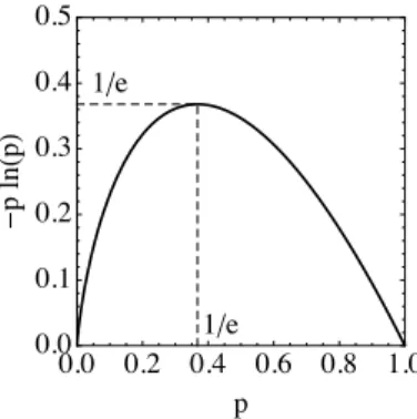
The entropy is seen to be a sum of functions of the form plog(p), wherep2[0,1].

The behavior of this function is shown in Fig.2.3. It tends to zero both whenp!0 and p! 1, and has a maximum at p =1/e. Hence, any state which has pk =0or pk=1 will not contribute to the entropy (even though log(0) alone diverges, 0 log(0) is well behaved). States that are too deterministic therefore contribute little to the entropy.

Entropy likes randomness.

Since each plog(p) is always non-negative, the same must be true forS(⇢):

S(⇢) 0. (2.54)

35

The generalization of ^{the Shannan entropy to density matrices}

is called the

^Neumann entropy

In terms of ^Xu

simply ^{get the}

Shannon entropy

Moreover, if the system is in a pure state,⇢=| ih |, then it will have one eigenvalue p1=1 and all others zero. Consequently, in a pure state the entropy will be zero:

The entropy of a pure state is zero. (2.55)

In information theory the quantity log(pk) is sometimes called thesurprise. When an

“event” is rare (pk ⇠0) this quantity is big (“surprise!”) and when an event is common (pk⇠1) this quantity is small (“meh”). The entropy is then interpreted as theaverage surpriseof the system, which I think is a little bit funny.

��� ��� ��� ��� ��� ���

���

���

���

���

���

���

�

-���(�)

�/�

�/�

Figure 2.3: The function plog(p), corresponding to each term in the von Neumann en- tropy (2.53).

As we have just seen, the entropy is bounded from below by 0. But if the Hilbert space dimensiondis finite, then the entropy will also be bounded from above. I will leave this proof for you as an exercise. What you need to do is maximize Eq. (2.53) with respect to thepk, but using Lagrange multipliers to impose the constraintP

kpk =1.

Or, if you are not in the mood for Lagrange multipliers, wait until Eq. (??) where I will introduce a much easier method to demonstrate the same thing. In any case, the result is

max(S)=log(d). Occurs when ⇢= I

d. (2.56)

The entropy therefore varies between 0 for pure states and log(d) for maximally disor- dered states. Hence, it clearly serves as a measure of how mixed a state is.

Another very important property of the entropy (2.53) is that it is invariant under unitary transformations:

S(U⇢U^†)=S(⇢). (2.57)

This is a consequence of the infiltration property of the unitariesU f(A)U^†= f(UAU^†) [Eq. (1.58)], together with the cyclic property of the trace. Since the time evolution of closed systems are implemented by unitary transformations, this means that the entropy is a constant of motion. We have seen that the same is true for the purity:

unitary evolutions do not change the mixedness of a state. Or, in the Bloch sphere

36

picture, unitary evolutions keep the state on the same spherical shell. For open quantum systems this will no longer be the case.

As a quick example, let us write down the formula for the entropy of a qubit. Recall the discussion in Sec.2.4: the density matrix of a qubit may always be written as in Eq. (2.19). The eigenvalues of ⇢are therefore (1±s)/2 where s = q

s²_x+s²_y+s²_z represents the radius of the state in Bloch’s sphere. Hence, applying Eq. (2.53) we get

S =

✓1+s 2

◆log✓1+s 2

◆ ✓1 s 2

◆log✓1 s 2

◆

. (2.58)

For a pure state we haves = 1 which then givesS = 0. On the other hand, for a maximally disordered state we haves=0 which gives the maximum valueS =log 2, the log of the dimension of the Hilbert space. The shape ofSis shown in Fig.2.4.

��� ��� ��� ��� ��� ���

���

���

���

���

���

���

���

���

�

�(ρ)

��(�)

Figure 2.4: The von Neumann entropy for a qubit, Eq. (2.58), as a function of the Bloch-sphere radiuss.

The quantum relative entropy

Another very important quantity in quantum information theory is thequantum relative entropyorKullback-Leibler divergence. Given two density matrices⇢and , it is defined as

S(⇢|| )=tr(⇢log⇢ ⇢log ). (2.59) This quantity is important for a series of reasons. But one in particular is that it satisfies theKlein inequality:

S(⇢|| ) 0, S(⇢|| )=0 i↵⇢= . (2.60)

The proof of this inequality is really boring and I’m not gonna do it here. You can find it in Nielsen and Chuang or even in Wikipedia.

37

Eq. (2.60) gives us the idea that we could use the relative entropy as a measure of thedistancebetween two density matrices. But that is not entirely precise since the relative entropy does not satisfy the triangle inequality

d(x,z)d(x,y)+ +d(y,z). (2.61) This is something a true measure of distance must always satisfy. If you are wondering what quantities are actual distances, thetrace distanceis one of them²

T(⇢, )=||⇢ ||1:=tr q

(⇢ )^†(⇢ ). (2.62)

But there are others as well.

Entropy and information

Define the maximally mixed state⇡ =Id/d. This is the state we know absolutely nothing about. We have zero information about it. Motivated by this, we can define the amount of information in a state⇢as the “distance” between⇢and⇡; viz,

I(⇢)=S(⇢||⇡).

But we can also open this up as

S(⇢||1/d)=tr(⇢log⇢) tr(⇢log(Id/d))= S(⇢)+log(d).

I know it is a bit weird to manipulateId/dhere. But remember that the identity matrix satisfiesexactlythe same properties as the number one, so we can just use the usual algebra of logarithms in this case.

We see from this result that the information contained in a state is nothing but

I(⇢)=S(⇢||⇡)=log(d) S(⇢). (2.63)

This shows how information is connected with entropy. The larger the entropy, the less information we have about the system. For the maximally mixed stateS(⇢)=log(d) and we get zero information. For a pure stateS(⇢) = 0 and we have the maximal information log(d).

As I mentioned above, the relative entropy is very useful in proving some mathe- matical relations. For instance consider the result in Eq. (2.56). If we look at Eq. (2.63) and remember thatS(⇢|| ) 0, this result becomes kind of obvious:S(⇢)log(d) and S(⇢)=log(d) i↵⇢=1/d, which is precisely Eq. (2.56).

2The fact that⇢ is Hermitian can be used to simplify this a bit. I just wanted to write it in a more general way, which also holds for non-Hermitian operators.

38

Respansefenctions

A very

problem ⁱⁿ statistical mechanics

that of measuring ^the response of

system ^to

^{certain external}

stimulus ^{This is} usually ^formulated

^follows

^have

^system

with Hamiltonian ^Ho

^then apply

^stimulus

^{which couples}

to ^some operator ^{A such that the} Hamiltonian changes ^to

H

231

of

^the coupling doesn't have to be like this But this ^kind

of coupling ^{terms out}

^be quite ^{common the most} important

example ^{is that of}

^{spin system ecerpled to}

magnetic ^field

that _{H Ho} h Sz

I

will work ^{with 237} for

though ^because

want ^to emphasize ^{that the results}

^also

^beyond spin systems

the quantity

^{want to evaluate}

^{the response of the} system ^{to the stimulus}

ay

tr

P't

tr

PH

what

want ^{to show in that this}

^{be written}

sA

where ^F

Z

You already ^showed

^{in the problem set for the}

^{of spin}

But ^here

^{would like to go} through

careful proof ^because

there ^is actually

^{subtlety involved related to whether}

^{not A}

and Ho commute

The

^is that ^{in order to write} something ^like

need ^to

pete _pH

2

2h

If ^{Ho A}

^then

^write

e

pH

^PHO epXA

In thin

e

P't

P'to epia

and ₂ ERA _p ^{A EP A EP} PA

22

since A commutes ^with itself ^Then

p ^A

PH when Ho A

zz

2,2

BH

so

that going from ^{251 to}

^easy

a

f ^{Z Fent} If

But if ^H

^to competing ²

PHI ^2x

^{not trivial Quite}

surprisingly

though Eq ^{267 continues to hold Let's}

why

It

useful

^{have the} following ^{BCH expansion}

^mind

let Kcx denote

arbitrary ^{operator then}

eN _dd f

^dd tz ⁴

^{d 3}

you

verify ^this formula ^{by series} expanding ^the exponentials ⁱⁿ

both sides ⁱⁿ

Taylor ^series

287

shows

that

compete de ^it matters whether

what ^DX

or

not dI commutes ^with

^If they

^{then it's easy If they}

DX

don't ^then

set

^tin principle ^{infinite series}

For

problem ^KC

^{p Ho}

^{p XA}

^{21 pa}

we

then get

2x

a

P't PA I

^{PA CK CK PA}

PH Ca

But

^comes the fun part ^{let's earmpute}

tr If

^{P't tr pa}

^{PH Iz}

tr Ex pa

^B't

30

what _want

tr Ex pa

^P J

Using ^the cyclic ^{property of the trace}

^{write the End}

team

tr Capa

^tr f

^{p A}

^{tr PA}

tr pa

^tr panek

0

since

^and

earmmute ^the

^{also true for all other}

serums in ¹²⁸ Thus

reach ^the quite ^nice conclusion that

tr eBH ptr ^{AEBH csi}

the derivation of ^{126 therefore renren.ms unaltered}

^if

A

and

Ho

not commute

Susceptibility

the susceptibility ^{is defined}

^the sensitivity of

^to

changes ⁱⁿ

X ^2C

132

Ilugging ^{in the} definition ^of

^{together with}

X I trfA P

2X fr

pH

22

ad ^{tr ca}

^BH trae

z

2X

Iz ^{tr CA}

^{PH p CA}

2

The first ^term

^bit tricky ^{If Ho}

^{277 to} get

X f ^{tr AZ}

^{PH p a}

2

Z

pfcA7 ¹³³

thin result ^is quite ^{nice It shows that the} susceptibility ^the sensitivity ^{of CA to changes in X is} actually ^{related to the}

variance of ^{a ie to the} fluctuations ^{of A ins} equilibrium

when Ho ^A to Eq ³³

^{longer holds In this}

^it

in useful ^to

^the following ^Feymmann integral tricky

a ^e

B pojds

^PHS Aep ^Hs

^{PH gu}

Thin identity ^is actually

consequence of ^{1287 It is}

demonstrated

in the appendix ^below

^{then get}

X Tf ^{as tr A}

^{PASA EPH}

PH p ^ca

or

x.io

EPAeP ^{A 1352}

If ^Ho

^thin clearly ^{reduces to 133 But written like this}

it

clearly ^{shows how He A f}

affects ^X

The susceptibility

defined ^for any ^{X However} suite ^often

interested ^{in the value of}

^{gov X}

^this

is

linear response theory

we

apply

infinitesimal perturbation ^and analyze ^{how the}

system ^{responds to it To leading}

order

may ^{in thin}

compete

X from ^the unperturbed ^{state Ho}

X

p f ^{jds A}

^{PHOSA EPH's AI go}

where So ^tr C EP Izo

^thermal average

^the

unperturbed

Hamiltonian ^Ho

App fymmmti

gwihded.tw

e

discussed ⁱⁿ Eq ^{267 the following BCH} expansion

dote ^dd ECK IF j.cn ^{a If 33}

^ca

we can

rewrite ^{this in terms} of

integral identity

^to

Feynman ^which

^be quite ^{useful To}

^{that recall the}

traditional

BC it expansions

e

y

Yt ^x y ^X Ex Y ^CA

comparing ^{with CA}

^{that the} coefficients

^{bit off}

For instance

^{CA 7 the} factor ^{of Yz multiplies K}

^whereas

in ca

it multiplies

^{EX YJ}

We ^can

fix ^this by introducing

armillary ^integrals

first

f

^Jds

since

ds

42 Continuing ^{in the}

^way

K

Ek

Jds

^Cri

I'm ^not doing anything ^{with the operators} just ^{playing with}

the coefficients

Eg ^{CA I may then be rewritten}

u

daff ^{ds K SEK}

k ⁱ

k En

^e

and if

^{earmpane thin with CA 27}

we see

that the

integrand ^{is precisely in the usual BCH forum}

d Jds

^de _di

^{e k}

changing

^s

alternatively ^{write this}

K

KS KS

dd

fois

^DI _di

0

Thus ^to summarize

ddzek

ejodseksdye

ekfdse ksdd.IE ^ca

If

^K

^then

cancel out ^e

^with

^KS leading

to K

dde DI ^e

DX

otherwise

^{have to} stick with ^{A 3}