locally convex curves in the sphere
Nicolau C. Saldanha August 29, 2013
Abstract
A smooth curveγ : [0,1]→S2 is locally convex if its geodesic curvature is positive at every point. J. A. Little showed that the space of all locally convex curves γ with γ(0) =γ(1) =e1 and γ′(0) = γ′(1) = e2 has three connected componentsL−1,c,L+1,L−1,n. The spaceL−1,c is known to be contractible. We prove that L+1 and L−1,n are homotopy equivalent to (ΩS3)∨S2∨S6 ∨S10∨ · · · and (ΩS3)∨S4 ∨S8∨S12∨ · · ·, respectively.
As a corollary, we deduce the homotopy type of the components of the space Free(S1,S2) of free curves γ : S1 → S2 (i.e., curves with nonzero geodesic curvature). We also determine the homotopy type of the spaces Free([0,1],S2) with fixed initial and final frames.
1 Introduction
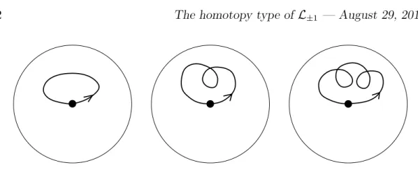
A curveγ : [0,1]→S2is calledlocally convex if its geodesic curvature is always positive, or, equivalently, if det(γ(t), γ′(t), γ′′(t))>0 for allt. LetLI be the space of all locally convex curves γ with γ(0) =γ(1) = e1 and γ′(0) = γ′(1) =e2; the precise topology for this space of curves will be discussed in the paper. J. A. Little [15] showed thatLI has three connected componentsL−1,c,L+1,L−1,n; examples of curves in each connected component are shown in Figure 1.
The connected componentL−1,c can be defined to be the set of simple curves inLI: the space L−1,c is known to be contractible ([1] and [25], Lemma 5). The aim of this paper is to determine the homotopy type of the two remaining spaces L+1 and L−1,n. Our main result is the following.
2000Mathematics Subject Classification. Primary 53C42; Secondary 34B05, 57N20, 53C29.
Keywords and phrasesConvex curves, topology in infinite dimension, periodic solutions of linear ODEs.
1
Figure 1: Curves in L−1,c, L+1 and L−1,n.
Theorem 1 The components L+1 and L−1,n are homotopically equivalent to (ΩS3)∨S2 ∨S6 ∨S10∨ · · · and (ΩS3)∨S4∨S8∨S12∨ · · ·, respectively.
Here ΩS3 is the space of loops in S3, i.e., the set of continuous maps α : [0,1] → S3 with α(0) = α(1) = 1, where 1 ∈ S3 is a base point, with the C0 topology. A more careful description of the connected componentsL+1andL−1,n
is given below.
A motivation for considering these spaces comes from differential equations.
Consider the linear ODE of order 3:
u′′′(t) +h1(t)u′(t) +h0(t)u(t) = 0, t ∈[0,1];
the set of pairs of potentials (h0, h1) for which the equation admits 3 linearly inde- pendent periodic solutions is homotopically equivalent toLI. The corresponding problem in order 2 is much simpler ([5], [6], [21]).
Alternatively, in Gromov’s language ([11], [7]), given two smooth Rieman- nian manifolds Vn and Wq, a map f : Vn → Wq is free (or second order free) if the second order osculating space is non-degenerate (we use covariant deriva- tives); let Free(V, W) be the space of such free maps. Perhaps the simplest non-trivial example here is Free(S1,S2), the space of curves γ : S1 → S2 with det(γ(t), γ′(t), γ′′(t)) 6= 0 for all t. Thus Free(S1,S2) differs from our space LI only by the fact that in Free(S1,S2) negative determinants are allowed, as are arbitrary initial frames Q∈SO3. The following result is a direct consequence of Theorem 1.
Corollary 1.1 The space Free(S1,S2) has six connected components, with two homotopically equivalent to each of the following spaces:
SO3× L−1,c ≈SO3,
SO3 × L+1 ≈SO3× (ΩS3)∨S2 ∨S6 ∨S10∨ · · · , SO3× L−1,n ≈SO3× (ΩS3)∨S4∨S8∨S12∨ · · ·
.
Recall that if q > n(n+3)2 then free maps satisfy the parametrical h-principle;
we are here in the critical case n = 1 and q = n(n+3)2 = 2 and the principle (incorrectly applied) would predict a (wrong) simpler answer. This paper does not require any familiarity with these ideas but the reader may notice that ideas similar to the h-principle will play an important part.
These spaces and variants have been discussed, among others, by B. Shapiro, M. Shapiro and B. Khesin ([24], [23]). These spaces are also the orbits of the second Gel’fand-Dikki brackets and therefore have a natural symplectic structure ([9], [10]). Furthermore, these spaces are related to the orbit classification of the Zamolodchikov Algebra ([13], [17]); these interpretations shall not be used or discussed in this paper.
Although the above authors ponder about the interest of understanding the topology of such spaces, their results deal mostly with π0, i.e., with counting and identifying connected components. The present author has also previously proved some weaker results about the topology of these spaces, regarding the fundamental group and the first few (co)homology groups ([18], [19]); these results are now of course easy consequences of Theorem 1.
Corollary 1.2 The spaces L+1 and L−1,n are connected and simply connected and, for k >0, their cohomology is given by
Hk(L+1;Z) =
0, k odd, Z2, 4|(k+ 2), Z, 4|k;
Hk(L−1,n;Z) =
0, k odd, Z, 4|(k+ 2), Z2, 4|k.
LetI be the space of immersions γ : [0,1]→S2 (of class Ck for some k ≥2) withγ′(t)6= 0,γ(0) =e1,γ′(0) =e2. LetL ⊂ I be the subspace of locally convex curves; thus, for γ ∈ I we haveγ ∈ L if and only if det(γ(t), γ′(t), γ′′(t))>0 for allt. For each γ ∈ I, consider its Frenet frame Fγ : [0,1]→SO3 defined by
γ(t) γ′(t) γ′′(t)
=Fγ(t)R(t),
R(t) being an upper triangular matrix with (R(t))11 > 0 and (R(t))22 > 0 (the left hand side is the 3×3 matrix with columns γ(t), γ′(t) and γ′′(t)). In other words, the first column of Fγ(t) is γ(t), the second is the unit tangent vector tγ(t) =γ′(t)/|γ′(t)| and the third column (which is now uniquely determined) is the unit normal vectornγ(t) = γ(t)×tγ(t). For Q∈SO3, let IQ ⊂ I be the set of curvesγ ∈ I for which Fγ(1) =Q; similarly, let LQ =L ∩ IQ.
The universal (double) cover of SO3 is S3 ⊂ H, the group of quaternions of absolute value 1; let Π : S3 → SO3 be the canonical projection. For γ ∈ I, the
curve Fγ can be lifted to define ˜Fγ : [0,1] → S3 with ˜Fγ(0) = 1, Π◦F˜γ = Fγ. The value of ˜Fγ(1) partitions IQ as a disjoint union Iz ⊔ I−z: here Π(±z) = Q and γ ∈ Iz if and only if ˜Fγ(1) = z; similarly, letLz =LΠ(z)∩ Iz. Notice that if γ is a simple curve in II then ˜Fγ(1) = −1 and therefore γ ∈ I−1. We can now more precisely describe the three connected components of LI: the component L+1 is a special case of this definition and L−1 has two connected components L−1,c (convex or simple curves) and L−1,n (non-simple).
A locally convex curveγ : [t0, t1] → S2 is convex if γ intersects any geodesic (great circle) at most twice. This definition requires a couple of clarifications.
First, endpoints do not count as intersections so, for instance, a simple closed locally convex curve is convex. Second, intersections are counted with multiplicity so that a tangency counts as two intersections. It follows from the definition that convex curves are simple. In this paper we will see other equivalent definitions.
A matrixQ∈SO3 isconvex if there exists a convex arcγ ∈ LwithFγ(1) =Q.
We shall see that the subset ofSO3 of convex matrices is the disjoint union of one of the top dimensional Bruhat cells and a few lower dimensional cells contained in its closure. Similarly, a quaternion z ∈ S3 is convex if there exists a convex arc γ ∈ L with ˜Fγ(1) =z. It is not hard to see that if −z is convex thenz is not.
We can now state a more general version of our main theorem. Herei∈S3 is the usual quaternion. Notice that −1 is convex but1, iand −i are not.
Theorem 2 Let z ∈ S3. Then the space Lz is homotopically equivalent to L−1 if z is convex, L1 if −z is convex and Li otherwise. Moreover, the following homotopy equivalences hold:
L−1 ≈(ΩS3)∨S0∨S4∨S8∨ · · · ; L+1 ≈(ΩS3)∨S2∨S6∨S10∨ · · · ; Li ≈ΩS3. We prove Theorem 2 not just for the sake of proving a stronger statement but mainly because it is not clear how to produce a complete proof of Theorem 1 (whose statement is simpler and more natural) without strong use of Bruhat cells and other algebraic notions. By the time these ideas have been mastered, both theorems are proved simultaneously.
Let ΩzS3 be the space of continuous curvesα: [0,1]→S3,α(0) =1,α(1) =z:
this is easily seen to be homeomorphic to ΩS3 and the two spaces shall from now on be identified. We just constructed the map ˜F : Iz → ΩzS3, γ 7→ F˜γ. It is a well-known fact (which follows from the Hirsch-Smale Theorem) that this map is a homotopy equivalence ([16], [12], [26]). Theorem 2 implies that the inclusions i:Lz → Iz are homotopy equivalences only for certain quaternions z.
We now proceed to give an overview of the paper and of the proof of the main theorems. Section 2 addresses the rather technical issue of what, precisely, is the best topology for the spaceLz. As we shall see, we may allow for the juxtaposition of curves (provided their Frenet frames agree); on the other hand, when desirable,
we may assume curves to be smooth. In Section 3 we apply the construction of Bruhat cells to our scenario. We also study projective transformations. The short Section 4 collects a few useful facts about the total (euclidean) curvature of spherical curves.
It follows from Little’s results that a circle drawn twice and a circle drawn four times are in the same connected component of LI. In Section 5 we give a careful description of a path joining these two curves. We also prove a few facts about this path which will be needed later.
As we have just mentioned, the inclusioni:Lz → Iz need not be a homotopy equivalence. In Section 6 we see that half of the story, so to speak, still holds.
Proposition 1.3 Let z ∈ S3. For any compact space K and any function f : K → Iz there exists g : K → Lz and a homotopy H : [0,1]×K → Iz with H(0, p) =f(p) and H(1, p) =g(p) for all p∈K.
The maps i:Lz → Iz therefore induce surjective maps πk(Lz)→πk(Iz).
In a nutshell, if a curve has very large (positive) geodesic curvature it looks like a phone wire and we call it sufficiently loopy. Any compact family α0 : K → Iz can be approximated in the C0 topology by a family α1 : K → Iz of sufficiently loopy (and therefore locally convex) curves (in Figure 2, γ0 =α0(p) and γ1 = α1(p) for some p ∈ K). Also, families of sufficiently loopy curves can be deformed without losing the property of being locally convex.
Figure 2: Curvesγ0 ∈ I±1 (thick) and γ1 ∈ L±1 (thin).
The difficulty in proving (the false fact) that the inclusion Lz ⊂ Iz is a homotopy equivalence is that there is no uniform procedure to add loops to locally convex curves within the set of locally convex curves.
In Section 7 we introduce a crucial construction in our discussion: a curve γ ∈ LQ is multiconvex of multiplicity k if it is the juxtaposition of k−1 simple closed convex curves with a finalk-th convex curve in LQ (see Figure 3).
We prove in Lemma 7.1 that, given Q, the closed subset Mk ⊂ LQ of mul- ticonvex curves of multiplicity k is either empty or a contractible submanifold
Figure 3: Two multiconvex curves of multiplicity 3
of codimension 2k − 2 with trivial normal bundle. Assuming −z convex, we next construct in Lemma 7.3 maps h2k−2 : S2k−2 → L(−1)kz which intersect Mk transversally and exactly once and are homotopic to a constant as maps S2k−2 → I(−1)kz (details of the construction of the path in Section 5 are used here to verify thath2k−2 has the desired properties). Intersection with Mkshows that h2k−2 is not homotopic to a constant as a map S2k−2 → LI and there- fore defines a non-trivial element of the homotopy group π2k−2(L(−1)kz) which is taken to zero by the inclusion in I(−1)kz. Furthermore, intersection with Mk defines an element of the cohomology group H2k−2(L(−1)kz) not in the image of i∗ :H∗(I(−1)kz)→H∗(L(−1)kz) (compare with [18] and [19]). This does not prove our main theorem yet but already shows that if either z or −z is convex thenLz is not homotopically equivalent to Iz.
In Section 8 we introducegrafting, a process under which loops can sometimes be added to curves. In Section 9 we define thenext step function and learn to tell apart good and bad steps; Bruhat cells are essential here. Let Yz =LzrS
kMk
be the set ofcomplicated (i.e., not multiconvex) curves. The new tools introduced in Sections 8 and 9 are then used in Section 10 to understand the spaces Yz. Proposition 1.4 The inclusion Yz ⊂ Iz is a weak homotopy equivalence.
In order to determine the homotopy type of Lz, start with Yz and, for each k, add the set Mk. It follows from what we have proved that adding Mk (if nonempty) is equivalent to attaching a sphere S2k−2. These properties are then sufficient to complete, in Section 11, the proof of Theorems 1 and 2.
The author would like to thank Dan Burghelea, Boris Khesin, Boris Shapiro and Pedro Z¨uhlke for helpful conversations and the referee and editor for valuable contributions; thanks also go to the referee of [18] and [19] for encouragement towards considering the problem discussed in this paper. The author thanks the kind hospitality of the Mathematics Department of The Ohio State University during the winter quarters of 2004 and 2009 and of the Mathematics Department of the Stockholm University during his visits to Sweden in 2005 and 2007. The author also gratefully acknowledges the support of CNPq, Capes and Faperj (Brazil).
2 Topology of L
QWe now attack a rather technical problem: defining the best topological structure for the spaces LQ and IQ.
It turns out that different topological structures obtain different spaces which are however homotopically equivalent. The Ck metric for some k ≥2 is a rather natural choice but it has the inconvenience that when constructing a homotopy we prefer not to be distracted by the necessity to smoothen out certain points of our curves (we want to be allowed, for instance, to consider a curveγ which is a juxtaposition of arcs of circle).
Given a smooth immersionγ : [0,1]→S2, letγ′(t) = vγ(t)tγ(t) wherevγ(t) =
|γ′(t)|>0 and tγ(t) is the unit tangent vector to γ. Let nγ(t) =γ(t)×tγ(t) be the unit normal vector to γ, so that
t′γ(t) =−vγ(t)γ(t) + ˆvγ(t)nγ(t), n′γ(t) =−vˆγ(t)tγ(t)
where ˆvγ(t) = κγ(t)vγ(t), κγ(t) being the geodesic curvature of γ. The curve γ is locally convex if and only if ˆvγ(t)>0 for all t. In matrix notation, γ(t),tγ(t) and nγ(t) are the columns of the orthogonal matrix Fγ(t) which satisfies
F′γ(t) =Fγ(t)Λγ(t); Λγ(t) =
0 −vγ(t) 0 vγ(t) 0 −vˆγ(t)
0 ˆvγ(t) 0
.
Let V ⊂ so3 be the plane (i.e., 2-dimensional real vector space) of matrices M with (M)31= 0; Λγ can be considered a function from [0,1] toV. LetVI ⊂V be the half-plane (M)21 > 0; Λγ can also be considered a function Λγ : [0,1]→ VI. Conversely, given a smooth function Λγ : [0,1]→VI or, equivalently, vγ and ˆvγ, the above equations together with Fγ(0) = I may be interpreted as an initial value problem defining Fγ(t) and thereforeγ(t) = Fγ(t)e1.
Our aim is to consider a reasonably large space of functions which still allows the initial value problem above to be solved. The Hilbert space L2([0,1]) is now a natural choice: for v,ˆv ∈L2([0,1]) the initial value problem can be solved. We therefore interpretIQ to be the closed subset of (L2([0,1]))2 of pairs of functions (w,v) such that the solution Γ : [0,ˆ 1]→SO3 of the initial value problem
Γ′(t) = Γ(t)Λ(t), Γ(0) =I, (1)
satisfies Γ(1) =Q, where
Λ(t) =
0 −v(t) 0 v(t) 0 −v(t)ˆ
0 v(t)ˆ 0
, v(t) = w(t) +p
(w(t))2+ 4 2
(we have w(t) = v(t)−1/v(t), v(t) >0). The fact that Λ(t) belongs to the Lie algebra so3 guarantees that Γ(t) assumes values in the corresponding Lie group SO3. Also, the function Γ defined above is continuous, absolutely continuous and differentiable almost everywhere. In this way IQ ⊂(L2([0,1]))2 is a smooth Hilbert manifold of codimension 3. Indeed, consider the map ωI : (L2([0,1]))2 → SO3 taking (w,v) to Γ(1), where Γ : [0,ˆ 1] →SO3 is defined by the initial value problem (1) above. Smooth dependence on parameters tells us that this map is smooth; let us compute its derivative.
In general, for a curve Γ : [0,1]→ SO3, write Γ(t0;t1) = (Γ(t0))−1Γ(t1). Let L be a one-parameter family of functions L(s) : [0,1] → VI, s ∈ (−ǫ, ǫ) with L(0) = Λ. Let G(s) : [0,1]→SO3 be the solution of
(G(s))′(t) = (G(s))(t)(L(s))(t), (G(s))(0) =I
so that G(0) = Γ; notice that the derivative in this initial value problem is with respect to t. An easy computation gives that the derivative of G (with respect to s) satisfies
(G′(s))(t)(G(s)(t))−1 = Z t
0
(G(s))(τ)(L′(s))(τ)((G(s))(τ))−1dτ.
Assume, for instance, that (L′(0))(t) consists of three smooth narrow bumps around times ti so that
(Γ(1))−1(G′(0))(t)≈X
i
(Γ(ti; 1))−1(L′(0))(ti)Γ(ti; 1).
An easy computation shows that the spaces (Γ(ti; 1))−1VΓ(ti; 1) ⊂ so3 are not constant and therefore (Γ(1))−1(G′(0))(t) may assume any value in so3. The derivative of ωI is therefore surjective. The mapωI is thus a submersion andIQ
a regular level set. The geometric description ofIQ comes from the identification (w,v)ˆ ↔γ, whereγ(t) = Γ(t)e1.
Similarly, let VL ⊂ V ⊂ so3 be the quarter-plane (M)31 = 0, (M)32 > 0, (M)21 > 0. If γ is locally convex then the image of Λγ is contained in VL and, conversely, given a smooth function Λ : [0,1]→VL, equation (1) obtains a locally convex curve. Define LQ ⊂ (L2([0,1]))2 to be the set of pairs (w,w) such thatˆ (w,v)ˆ ∈ IQ where
ˆ
v(t) = w(t) +ˆ p
( ˆw(t))2+ 4
2 .
As above, define ω : (L2([0,1]))2 → SO3 taking (w,w) to Γ(1), where Γ is againˆ defined by equation (1). The computation above also shows that the smooth map ω is a submersion and LQ is a smooth Hilbert submanifold of codimension 3 in (L2([0,1]))2. We have a natural injective map LQ → IQ taking (w,w) to (w,ˆ v).ˆ
In the spirit of considering LQ and IQ to be sets of curves we call this map an inclusion (even though it is not an isometry with the above metric).
The spaceLQwe just defined is rather large. The spaceL[CQk]of locally convex curves of classCk (k≥2) is now naturally identified to a dense subsetL[CQk]⊂ LQ
with a different topology. But are these two spaces similar? Or, more precisely, is the inclusion a weak homotopy equivalence? The answer here is yes.
In order to see this, first consider L[[CQ k]], k ≥0, the subset of (Ck([0,1]))2 of pairs (w,w) such that Γ(1) =ˆ Q (where Γ is defined by the initial value problem (1)). The inclusion L[[CQ k]] ⊂ LQ is a homotopy equivalence: this follows directly from Theorem 2 from [4]. For the convenience of the reader, we quote here a simplified version of that result.
Proposition 2.1 Let X and Y be separable Banach spaces. Suppose i:Y →X is a bounded, injective linear map with dense image and M ⊂ X a smooth, closed submanifold of finite codimension. Then N = i−1(M) is a smooth closed submanifold of Y and the restriction i:N →M is a homotopy equivalence.
For k ≥ 1 the curves γ are now of class C2 and we may assume them to be parametrized by a constant multiple of arc length (this does not change the homotopy type of the space since the group of orientation-preserving diffeomor- phisms of [0,1] is contractible). In terms of the pairs (w,w), this says that weˆ may assumewto be constant. But for wconstant, ˆwis of class Ck if and only if γ is of classCk+2, completing the argument.
Summing up, and simplifying this discussion a little, we may assume our curves γ to be as smooth as our constructions require but when constructing a homotopy we may use curves for which the curvature is only piecewise continuous.
We will however try to be as consistent as reasonably possible in the use of the large spaceL defined above.
3 Projective transformations and Bruhat cells
In this section we present some more algebraic notation, especially the decompo- sition ofSO3 and S3 in (signed)Bruhat cells. Some of this material is presented in [20] in a more algebraic fashion and for arbitrary dimension.
The projective transformation π(A) : S2 → S2 associated to A ∈ SL3 is defined by π(A)(v) = Avc = (1/|Av|)Av. Similarly, define π(A) : SO3 → SO3
by π(A)(Q0) = Q1 if there exists U1 ∈ Up+3 with AQ0 = Q1U1; here Up+3 is the contractible group of upper triangular matrices with positive diagonal and determinant +1. In other words,π(A)(Q0) is obtained from AQ0 by performing Gram-Schmidt on columns. In particular, if A ∈ SO3 then π(A)(Q0) = AQ0.
This action of SL3 on SO3 is transitive but not doubly transitive; we shall soon discuss the extent to which it fails to be doubly transitive.
Notice thatπ(A) :S2 →S2 is an orientation preserving diffeomorphism. For an immersion γ : [0,1] → S2 define π(A)γ by (π(A)γ)(t) = π(A)(γ(t)); the curve π(A)γ is again an immersion. Since π(A) takes geodesics to geodesics, if γ : [0,1] → S2 is locally convex then so is π(A)γ (this can also be checked directly from the definition by a straightforward computation). The mapπ(A) is defined so that Fπ(A)γ =π(A)(Fγ) for any immersion γ : [0,1]→S2. Notice that π(A)I = I if and only if A ∈ Up+3. Thus, for U ∈ Up+3, π(U) defines a smooth map from LQ toLπ(U)Q.
LetB3 ⊂O3 be the Coxeter-Weyl group of signed permutation matrices: the group B3 has 48 elements and corresponds to the isometries of the octahedron of vertices ±e1,±e2,±e3. Let B+3 = B3 ∩SO3 be the subgroup of orientation preserving isometries. Dropping signs defines a homomorphism from B3+ to the symmetric group S3: the number of inversions of Q ∈ B3+ is the number of inversions of the corresponding permutation in S3 (recall that the number of inversions of π ∈ Sn is the number of pairs (i, j) with i < j and π(i) > π(j)).
We denote an element of B3+ by the letter P (for permutation), indicating in the subscript the corresponding permutation (as a cycle) and the signs, read by column, in binary:
0 = + + +, 1 = + +−, 2 = +−+, 3 = +− −, . . . , 7 =− − −; thus, for instance
P(13);1 =
0 0 −1
0 +1 0
+1 0 0
, P(13);2 =
0 0 +1 0 −1 0
+1 0 0
.
The lift ˜B3+ ⊂S3 ofB3+ is the group of 48 quaternions with either one coordinate of absolute value 1 and three equal to 0 or two coordinates of absolute value 1/√
2 and two equal to 0 or four coordinates of absolute value 1/2. As a subset of R4, B˜+3 is also the root systemF4 (with all vectors of size 1, unlike what is usual for Lie algebras). For instance,
Π
1−j
√2
=P(13);1, Π
i+k
√2
=P(13);2.
The Bruhat cell Bru(Q) ⊂ SO3 of Q ∈ SO3 is the set of all orthogonal matrices of the form U0QU1−1, with U0, U1 ∈ Up+3. Each Bruhat cell contains a unique element of B3+. We also denote the Bruhat cells by Bru∗, with subscripts defined as for P∗ ∈ B3+; thus, for instance, Bru(P(13);1) = Bru(13);1. The cell Bru(P) (P ∈B3+) is diffeomorphic to Rd, where d is the number of inversions of
P. There are therefore exactly four open cells, corresponding to the two matrices above plus
Π
1+j
√2
=P(13);4, Π
i−k
√2
=P(13);7.
IfQ0 andQ1 belong to the same Bruhat cell then there exists a canonical and explicit diffeomorphism between the Hilbert manifolds LQ0 and LQ1. Indeed, for Q0 and Q1 ∈ Bru(Q0) let U0, U1 ∈ Up+3 be such that U0Q0 = Q1U1; U0 is uniquely defined if we require U0 ∈ Up13, where Up13 ⊂ Up+3 is the subgroup of matrices with diagonal entries equal to +1. Then the mapπ(U0) :LQ0 → LQ1 is a diffeomorphism; its inverse is the similarly constructed map π(U0−1).
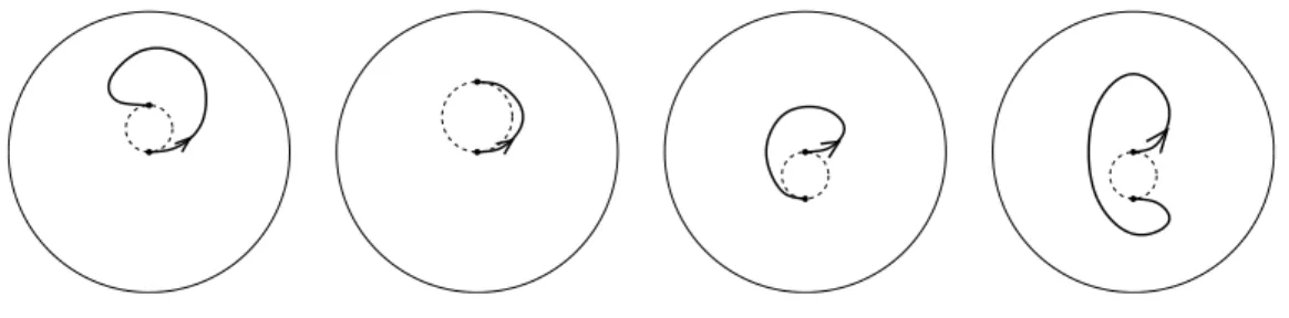
Figure 4 shows example of curves γ ∈ LQ for Q ∈ Bru(13);ℓ for ℓ = 1,2,4,7 (in this order).
Figure 4: Representatives of the open Bruhat cells
The dashed closed convex curves indicate a convenient geometric way to rec- ognize these Bruhat cells: in all cases there exists a closed convex curve tangent to both endpoints ofγ and orientations at the endpoints allow us to distinguish between cells.
For γ ∈ L, let Γ = Fγ : [0,1] → SO3 and write Fγ(t0;t) = Γ(t0;t) = (Γ(t0))−1Γ(t). Similarly, ˜Fγ(t0;t) = ˜Γ(t0;t) = (˜Γ(t0))−1Γ(t) where ˜˜ Γ : [0,1]→S3 is a lift of Γ. Clearly, Γ(0;t) = Γ(t), Γ(t0;t0) = I, ˜Γ(t0;t0) = 1. On the other hand, there existsǫ >0 such that for allt∈(t0, t0+ǫ) we have Γ(t0;t)∈Bru(13),2. A locally convex arc γ|[t0,t1] isconvex if Fγ(t0;t)∈Bru(13);2 for all t∈(t0, t1).
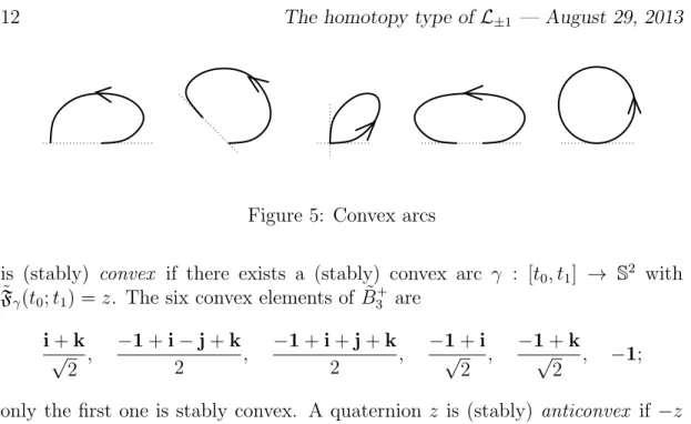
Notice that we do not require that Fγ(t0;t1) ∈ Bru(13);2; if this also happens thenγ isstably convex. There are five other Bruhat cells to whichFγ(t0;t1) may belong: Bru(123);6, Bru(132);0, Bru(23);2, Bru(12);4 and Brue;0 = I. Examples of convex arcs corresponding to these five cells are given in Figure 5. We shall come back to these five cells again and again.
Recall that a matrix Q ∈ SO3 is (stably) convex if there exists a (stably) convex arc γ : [t0, t1] → S2 with Fγ(t0;t1) = Q. Thus, the set of stably convex matrices is the open cell Bru(13);2 and the set of convex matrices is the union of the six Bruhat cells above (including the open cell). Also, a quaternion z ∈ S3
Figure 5: Convex arcs
is (stably) convex if there exists a (stably) convex arc γ : [t0, t1] → S2 with F˜γ(t0;t1) =z. The six convex elements of ˜B+3 are
i+k
√2 , −1+i−j+k
2 , −1+i+j+k
2 , −1+i
√2 , −1+k
√2 , −1;
only the first one is stably convex. A quaternion z is (stably) anticonvex if −z is (stably) convex. The sets of convex and anticonvex quaternions are unions of distinct Bruhat cells and therefore disjoint; furthermore, the only points of intersection between their respective closures are ±1.
Let Cν be the circle (contained in S2) with diameter e1e3, parametrized by ν1 ∈ LI,
ν1(t) = 1 2
1 + cos(2πt),√
2 sin(2πt),1−cos(2πt) for which
F˜ν1(t) = exp πtkˆ
, Λ˜ν1(t) = πkˆ, ˆk= i+k
√2 ,
where ˜Λγ(t) = (˜Fγ(t))−1F˜′γ(t). For a positive real number s, let νs(t) =ν1(st) so that νs ∈ Lexp(πsk)ˆ . In particular, for integer k > 0, νk ∈ L(−1)k. We also have ν1 ∈ L−1,c and νk ∈ L−1,n for k odd, k >1.
More generally, a circle of radiusρ < π/2 is a closed convex curve:
γ(t) = cos(2πt) sin(ρ)v1+ sin(2πt) sin(ρ)v2+ cos(ρ)v3, t∈[0,1],
where v1, v2, v3 is a positively oriented orthonormal basis. Thus, νs is a circle of radius π/4 (measured along the sphere).
The image of a convex circle by a projective transformation is a spherical ellipse, or just ellipse. Notice that for us an ellipse is an oriented curve. Also, a projective arc-length parametrization of an ellipse is a locally convex curve γ : [t0, t1]→S2 of the formγ =π(A)◦˜γwhereA∈SL3and ˜γis a parametrization by a multiple of arc length of a circle. We shall sometimes use ellipses when a concrete choice of convex arc is desirable.
Lemma 3.1 Let γ : [0,1]→S2 be a stably convex arc and let t ∈(0,1). Set F˜γ(0) =z0, γ(t) = vt, F˜γ(1) = z1.
Then there exists ǫ >0 such that if zˆ0 ∈S3, vˆt∈S2 and zˆ1 ∈S3 are such that
|zˆ0−z0|< ǫ, |vˆt−vt|< ǫ, |zˆ1 −z1|< ǫ
then there exists a unique ellipseE ⊂ˆ S2 and projective arc-length parametrization ˆ
γ : [0,1]→E ⊂ˆ S2 with
F˜γˆ(0) = ˆz0, γ(t) = ˆˆ vt, F˜γˆ(1) = ˆz1.
Proof: LetQi = Π(zi); draw inS2 geodesicsℓiperpendicular toQie3, oriented by Qie2 at Qie1 so that ℓi is tangent toγ at t=i(i= 0,1). Since z0−1z1 ∈Bru(13);2, the geodesics ℓ0 and ℓ1 are transversal and divide the sphere into four open regions, with the image ofγcontained in the region characterized by being to the left of both ℓ0 and ℓ1. Since all the relevant conditions are open, for sufficiently smallǫ >0 the corresponding geodesics ˆℓiare also transversal and ˆvtlies to the left of both ˆℓ0 and ˆℓ1. There exists A∈SL3 such that the projective transformation π(A) satisfies π(A) ˆQ0 = I and π(A) ˆQ1 = P(13);2; for sufficiently small ǫ > 0 we may furthermore assume that π(A)ˆvt lies in the first octant. There is c >0 such that, for
Bc =
c 0 0 0 c−2 0
0 0 c
,
π(BcA)ˆvt lies on the arc of circleν1 defined above, thus obtaining the desired arc of ellipse. Uniqueness follows from the fact that five points determine a conic and three points determine a projective transformation in the line.
Recall that two smooth curves osculate each other at a common point if they are tangent and have the same curvature at that point. The next lemma may be considered a limit case of the previous one.
Lemma 3.2 Let Q ∈ Bru(13);2; then there exists a unique ellipse E ⊂ S2 and projective arc-length parametrizationγ : [0,1]→ E ⊂S2 withγ convex,γ(0) =e1, γ′(0) =e2, E osculating the circle Ckˆ at e1 and Fγ(1) = Q.
Proof: As in the previous proof, there exists A ∈ SL3 with π(A)I = I and π(A)Q=P(13);2. WithBc as in the previous proof, the ellipsesγc =π(A−1Bc)◦ν1
satisfy γc(0) = e1, γc′(0) = e2, and Fγc(1) = Q; there exists a unique c > 0 for which γc oscullates Ckˆ. Uniqueness again follows from five points determining a
conic (oscullation counts as three points).
4 Total curvature
Given a locally convex curve γ : [a, b] → S2, let κγ : [a, b] → R be the geodesic curvature of γ. This must not be confused with the euclidean curvature κEγ of γ interpreted as a curve in R3: κEγ(t) = q
1 +κ2γ(t). The total (euclidean) curvature of γ : [a, b]→S2 is
tot(γ) = Z
[a,b]
κEγ(t)|γ′(t)|dt.
Notice that tot(νs) = 2πs.
Lemma 4.1 Let γ : [a, b]→S2 be a locally convex curve.
(a) The total curvature of γ equals the total variation of tγ and twice the length of F˜γ:
tot(γ) = Z
[a,b]|t′γ(t)|dt = 2 Z
[a,b]|F˜′γ(t)|dt.
(b) If γ ∈ LI is a closed convex curve then tot(γ)∈[2π,4π).
(c) If γ ∈ L is a convex arc then tot(γ)∈(0,4π].
(d) If tot(γ)< π then γ is convex.
The inequalities above are not necessarily the best possible.
Proof: Item (a) is a straightforward computation. The first inequality in item (b) is the well known general fact that the total curvature of a closed curve is at least 2π. Alternatively, given (a), ˜Γ = ˜Fγ : [0,1] → S3 satisfies ˜Γ(0) = 1, Γ(1) =˜ −1 so of course the length of ˜Γ must be at least π. For the second inequality in (b), first notice that κEγ(t)≤1 +κγ(t) so we must prove that
I1+I2 <4π, I1 = Z
[0,1]|γ′(t)|dt, I2 = Z
[0,1]
κγ(t)|γ′(t)|dt.
By Gauss-Bonnet, I2 = 2π−Aγ <2π, whereAγ is the area of the smaller disk in S2 bounded byγ. Letnγ : [0,1]→S2 be the unit normal vector: nγ(t) = Fγ(t)e3. A straightforward computation shows that
|n′γ(t)|=κγ(t)|γ′(t)|, κnγ(t) = 1/κγ(t).
Thus, again by Gauss-Bonnet, I1 =
Z
[0,1]
κnγ(t)|n′γ(t)|dt= 2π−Anγ <2π
where Anγ is (of course) the area of the smaller disk in S2 bounded by nγ. This completes the proof of (b).
For item (c), consider a convex arc γ : [0,1] → S2. For arbitrarily small ǫ > 0, γ|[0,1−ǫ] can be extended to a closed convex curve ˜γ. Thus, from (b), tot(γ|[0,1−ǫ])<tot(˜γ)<4π. Since this estimate holds for all ǫ, tot(γ)≤4π.
For item (d), assume thatγ1 : [a, b]→S2 is convex but that if the domain of γ1 is extended to define γ2 then γ2 is not convex. In other words, γ1 is similar to one of the curves in Figure 5. A case by case analysis shows that there exist t0 < t1 ∈[a, b] with tγ1(t1) =−tγ1(t0) and therefore
tot(γ1)≥ Z
[t0,t1]|t′γ1|(t)dt ≥π.
5 The map g
0The aim of this section is to construct a map g0 :S2 → L1 ⊂ I1. We shall have g0(s) =ν2 and g0(n) =ν4, where n= (0,0,+1) and s = (0,0,−1) are the north and south pole, respectively. The existence of such a map proves thatν2andν4are in the same connected component ofL1, consistently with Little’s result that LI has three connected componentsL−1,c,L1 and L−1,n (see Figure 1). As we shall see in Proposition 5.3,g0 turns out to be a generator of π2(I1)≈H2(I1;Z)≈Z. The map g0 is one the the crucial objects in this paper so its construction shall be discussed in some detail.
The map g0 is shown in Figure 6: here the bottom line is the south poles = (0,0,−1), the top line is the north polen= (0,0,+1) and other horizontal lines are circles contained in a plane of the form z =z0; vertical lines are meridians, i.e., half circles joining the two poles. Each small sphere is drawn here as a photo of a transparent sphere: a curve in the front is drawn a bit thicker. The vector perpendicular to the page pointing towards the reader is e1 +e3 with e3 −e1
pointing up and e2 to the right of the reader. The base point e1 is drawn as a thick dot.
Consider the equator of the unit sphere S2 contained in the plane z = 0.
Fix a unit normal vector N = (0,0,1) to the plane and call it up. Consider six equally spaced points P0 = P3 = (1/2,−√
3/2,0), Q0 = Q3 = (1,0,0), P1 = (1/2,√
3/2,0), Q1 = −P0, P2 = −Q0 and Q2 = −P1 along the equator.
Notice that Qi/2 is the midpoint of the segment PiPi+1. For α ∈ R, let ˜α = arcsin(sin(α)/2) so that ˜α∈[−π/6, π/6]. Let
Q±i (α) = cos(α−α)Q˜ i ±sin(α−α)N,˜
Figure 6: A sketch of g0 :S2 → L1.
so that Q+i (0) = Q−i (0) = Qi, Q−i (α) = Q+i (−α) and Q+i (a function of α) parametrizes the circle passing through ±Qi and ±N. Equivalently, Q+i (α) is the only point on the unit sphere such that the vector Q+i (α)− (Qi/2) is a positive multiple of (cosα)Qi+ (sinα)N. Let Ci±(α) be the circle containing Pi, Q±i (α) and Pi+1, so that Ci±(α) has radius cos(˜α) and is contained in a plane perpendicular to −cos(α)N ±sin(α)Qi. Let A±i (α)⊂ Ci±(α) be the arc from Pi
through Q±i (α) to Pi+1.
x
y N
P0
P1
P2 Q0
Q1
Q2
˜ α α
Qi Q+i (α)
Qi
2
Figure 7: Constructing Pi,Qi and Q+i (α).
Orient the circles Ci±(α) and the arcs A±i (α) from Pi through Q±i (α) to Pi+1. The circle Ci±(α) has geodesic curvature equal to ∓tan(˜α). Parametrize the arcs A+0(α), A−1(α), A+2(α), A−0(α), A+1(α), A−2(α) and A+0(α) by a mul- tiple of arc length using the domains [−1/12,1/12], [1/12,3/12], [3/12,5/12], [5/12,7/12], [7/12,9/12], [9/12,11/12] and [11/12,13/12], respectively. Concate- nate the above parametrizations to define a parametrization βα : [0,1] → S2 by a multiple of arc length of a curve Cα ⊂ S2. In particular, βα(0) = Q+0(α), βα(1/12) = P1, βα(2/12) = Q−1(α) and so on. Notice that βα is of class C1, even at the points t = j/12. The curve βα is an immersion; its geodesic cur- vature is always in the interval [−√
3/3,+√
3/3], with the extremes assumed for α=π/2+kπ,k ∈Z. The curveβ0is the equator covered twice;βπ is the equator covered four times with the opposite orientation. DefineBα=Fβα : [0,1]→SO3 as usual; lift this to define ˜Bα : [0,1]→S3with ˜B0(0) =1and ˜Bα(t) a continuous function ofα and t, 1-periodic in t and 4π-periodic in α.
Defineh = exp(πj/8); notice that hih−1 = ˆi= i−k
√2 , hkh−1 = ˆk= i+k
√2 . Define ˜Γα(t) = ˜Bα(t)h−1, Γα= Π◦Γ˜α and (of course)
γα(t) = Γα(t)e1 =Bα(t)e1+e3
√2 =
√2
2 βα(t) +
√2
2 nβα(t).
Geometrically, γα is the concatenation of six circle arcs ˜A±i , obtained fromA±i by increasing or decreasing the radius by π/4. The geodesic curvature of γα is
κγα(t) =
(tan π4 −α˜
, t∈[0,121)∪(123,125)∪(127,129)∪(1112,1], tan π4 + ˜α
, t∈(121,123 )∪(125,127 )∪(129,1112).
and therefore always in the interval [2−√
3,2+√
3], with extreme values assumed for α = π/2. Furthermore, tot(γα) is a strictly increasing function of α ∈ [0, π]
with tot(γ0) = 4π, tot(γπ) = 8π. Notice that Γ˜α
t+1
3
= exp 4π
3 k
Γ˜α(t); Γ˜α
t+ 1
2
=−Γ˜−α(t).
Define g0 :S2 → L1 by g0(p)(t) =
Γα
θ 6π
−1
γα
t+ θ 6π
, p= (cosθsinα,sinθsinα,−cosα).
Notice that g0 is well defined.
This construction yields the following result, due to Little ([15]); we state and prove it here in order to get used to the above construction which shall be needed later.
Lemma 5.1 Let n be a positive integer, n > 1. The curves νn and νn+2 are in the same connected component of LI.
Proof: The case n = 2 follows from the above construction of g0. For larger n, just consider νn as a concatenation of νn−2 with ν2, keep νn−2 fixed and apply the above construction to move from ν2 to ν4, thus obtaining a path in LI from
νn to νn+2.
We prove an auxiliary result concerning the curves βα and γα for later use.
A common oriented tangent to two oriented circles is an oriented geodesic which is tangent to both circles, with compatible orientation at tangency points. Thus, for instance, Ci±(α) and Ci+1∓ (α) are tangent at Pi+1; they also have a common oriented tangent, a geodesic passing throughPi+1. LetCk(resp. Ckˆ) be the great circle and subgroup of S3 of points of the form exp(sk) (resp. exp(sk)),ˆ s ∈ R. Recall that we write ˜Bα(t0;t1) = ( ˜Bα(t0))−1B˜α(t1).
Lemma 5.2 Let α∈(0, π).
(a) The common oriented tangents between two distinct circles among Ci±(α), i= 0,1,2, are the geodesics passing through the tangency point Pi+1 between Ci±(α) and Ci+1∓ (α), and only these.
(b) For t0, t1 ∈[0,1), if B˜α(t0;t1)∈ Ck then t0 =t1. (c) For t0, t1 ∈[0,1), if Γ˜α(t0;t1)∈ Cˆk then t0 =t1.
Proof: Recall that our circles Ci±(α) are not geodesics. Each circle therefore defines a disk (the smaller connected component of the complement).
For item (a), we have three essentially different pairs of circles to consider:
(C0+(α),C0−(α)), (C0+(α),C1+(α)) and (C0+(α),C1−(α)). In the first case, the two circles have opposite orientations and therefore the circles and corresponding disks would have to lie on opposite sides of a common oriented tangent. Since the open disks intersect, no common oriented tangent exists. In the second case orientations agree and therefore both disks would lie on the same side of a common oriented tangent. But the union of the two closed disks contains the arc from P0 through P1 to P2 and therefore is not contained in a hemisphere. Thus also in this case no common oriented tangent exists. Finally, in the third case again the two circles have opposite orientations and therefore the disks must lie on opposite sides of a common oriented tangent. But the closed disks touch at P1: the common oriented tangent must therefore pass through this point, completing the proof of the first claim.
For item (b), assume by contradiction that ˜Bα(t0;t1) = exp(sk), t0 6= t1. Consider the curve ˜Γ : [0,1]→S3 given by ˜Γ(t) = ˜Bα(t0) exp(2πtk). Notice that Γ(0) = ˜˜ Bα(t0) and ˜Γ(s/(2π)) = ˜Bα(t1). Also ˜Γ(t) = ˜Fγ(t) for γ the geodesic γ(t) = Bα(t0)(cos(4πt),sin(4πt),0). Thus γ is an oriented tangent to the curve Cα at two distinct points. These two points must belong to different circles Ci±
for a circle can not be twice tangent to the same geodesic. But this contradicts item (a).
Finally, for item (c), notice that
Γ˜α(t0;t1) =hB˜α(t0;t1)h−1 and therefore ˜Γα(t0;t1) = exp(sk) impliesˆ
B˜α(t0;t1) =h−1exp(skˆ)h= exp
sh−1khˆ
= exp(sk).
Thus item (b) implies item (c).
Proposition 5.3 The map g0 is a generator of π2(I1).
Proof: Given g : S2 → I1, define ˆg : S2 ×S1 → S3 by ˆg(p, t) = ˜Fg(p)(t), where we identify S1 = R/Z. Let N(g) be the degree of ˆg. Clearly N(g) is invariant by homotopy and N(g1∗g2) =N(g1) +N(g2) (where ∗ is the operation defining π2). We prove that |N(g0)|= 1, completing the proof of the proposition.
From Lemma 5.2 above, ˜Fg(p)(t) =1 implies either t = 0 orp=n (the north pole) and t = 1/2. For the purpose of computing the degree of ˆg0, we deform it to define another maph:S2×S1 →S3 corresponding to closed curves coinciding with g0(p) except at a small neighborhood of t = 0, where they cross the xz plane at a point (cos(ǫ),0,sin(ǫ)),ǫ >0. Thus the only preimage of 1 underh is (n,1/2) and we are left with verifying that it is topologically transversal.
Alternatively, again from Lemma 5.2 above, the preimages under ˆg0 of−1are exactly (s,1/2), (n,1/4) and (n,3/4). We are left with verifying that all three are topologically transversal and that the sign of the first is different from the sign of the last two, again implying |N(g0)|= 1.
Unfortunately,g0is not differentiable atsbut it does admit directional deriva- tives: that is enough. We go back to the construction of ˜Bα and ˜Γα in order to compute directional derivatives of g0. For t ∈ [−1/12,1/12], we may translate the geometric description above as:
B˜α(t) = expα 2j
exp (u(α)tk) exp (v(α)j), u(α) = 6 arccos cosα
p4−sin2α
!
, v(α) = −1 2arcsin
1 2sinα
.
Notice that u′(0) = 0, v′(0) = −1/4. Let ˜Bα•(t) be the derivative of ˜Bα(t) with respect to α; we have ( ˜B0(t))−1B˜0•(t) = w(t) where the auxiliary function w is defined by
w(t) = 1
4((2 cos(4πt)−1)j+ (−2 sin(4πt))i).
It is now easy to obtain similar formulas for other intervals and to deduce that ( ˜B0(t))−1B˜0•(t) =
(w(t−t0), t∈
t0− 121, t0+ 121
, t0 = k3,
−w(t−t0), t∈
t0− 121, t0+ 121
, t0 = k3 + 16, k ∈Z. Thus ( ˜B0(t))−1B˜0•(t), as a function oft, performs three full turns around the origin in the plane spanned by i and j. We now have that (B0(t;t+ 12))−1B0•(t;t+ 12) performs one full turn around the origin when t goes from 0 to 1/3.
Recall that ˜Γα(t) = ˜Bα(t)h−1 and therefore Γα(t;t+12) =hBα(t;t+12)h−1 and we have that (Γ0(t;t+ 12))−1Γ•0(t;t+12) performs one full turn around the origin when t goes from 0 to 1/3, but now in the plane spanned by ˆi and j. A similar computation shows that, when t goes from 0 to 1/3, (Γπ(t;t+ 12))−1Γ•π(t;t+ 12) also performs one full turn around the origin in the same plane.
Translating this back tog0 shows that whenpdescribes a small circle around either the south or the north pole,g0(p)(1/2) describes a small simple closed curve around (g0(s))(1/2) = (g0(n))(1/2) = e1, with (g0(p))′(1/2) ≈ (g0(s))′(1/2) =
(g0(n))′(1/2) = e2. The reader should check in Figure 6 that this is indeed the case: said simple closed curve is drawn clockwise when we go left to right along either the second row from the bottom (around s) or the second from the top (aroundn). It follows from Lemma 5.2 (and can be checked in Figure 6) that the same holds for other values of t. Thus, for instance, when p describes a left to right small circle around the north pole,g0(p)(1/4) and g0(p)(3/4) both describe simple closed curves arounde1, also oriented clockwise.
Finally, translating these results to ˆg0, the image under ˆg0 of a small sphere around (n,1/2) wraps once around1= ˆg0((n,1/2)), proving topological transver- sality at this point. Similarly, the image of a small sphere around (s,1/2), (n,1/4) or (n,3/4) wraps once around −1; the orientation is different for the first point because, from the point of view of S2, a left to right circle near n and a left to
right circle near s have opposive orientations.
6 Adding loops
In this section we present a few facts related to adding loops to a curve (or family of curves), including the proof of Proposition 1.3. This is of course similar to the proof of the Hirsch-Smale theorem ([12], [26]). The reader familiar with Gromov’s ideas will also recognize this as an easy instance of the h-principle ([7], [11]); others will be reminded of Thurston’s method for performing the sphere eversion by corrugations ([14]).
We need a precise version for the notion of adding n loops at a point t0 of a curve γ as in Figure 8. For γ ∈ I, t0 ∈ (0,1) and n a positive integer let γ[t0#n] ∈ I be defined by
γ[t0#n](t) =
γ(t), 0≤t≤t0−2ǫ;
γ(2t−t0+ 2ǫ), t0−2ǫ≤t≤t0−ǫ;
Fγ(t0)νn t−t0+ǫ 2ǫ
, t0−ǫ≤t≤t0+ǫ;
γ(2t−t0−2ǫ), t0+ǫ ≤t ≤t0+ 2ǫ;
γ(t), t0+ 2ǫ≤t ≤1;
here ǫ > 0 is taken sufficiently small. In words, we follow γ normally almost until t0: we then run a little in order to have room to insert νn (appropri- ately moved to the correct position), run a little again and then continue as γ.
Since reparametrizations of curves are not particularly interesting (the group of orientation-preserving diffeomorphisms of [0,1] is contractible) the precise value of ǫ is not particularly interesting either.


![Figure 8: Curves γ and γ [t 0 #n] .](https://thumb-eu.123doks.com/thumbv2/123dok_br/17631652.4197967/22.918.246.722.103.300/figure-curves-γ-γ-t-n.webp)


