Looking back at the US Great Inflation of the 1970s, we can see signs of what is to come in the expectations data. Third, it looks at a case where inflation has declined, instead of up, the American experience of the early 1980s. Most accounts of the sources of the Great Inflation see its origins during this time.
In fact, disposable income rose between the peak and trough of the recession, when the 1968 tax credit expired and the automatic stabilizers in the welfare state kicked in.
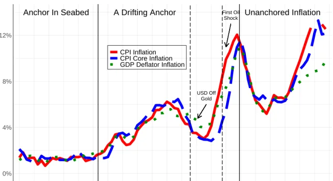
From 1971 to 1974: The anchor adrift
An auto workers' strike in 1971 reinforced this view, and the Federal Reserve's annual report was filled with analyzes of unit labor costs. One of the factors behind this change was political influence on monetary policy.
Conclusion: Expectations as add-factors
The inflation bias that yielded to political pressure on expectations given repeat elections was rejected, and yet it was evident in the data for the two decades that followed (Alesina, 1988). Neither of these options is very useful when trying to determine whether inflation expectations are anchored in the present.
3 Data on inflation expectations
- Inflation expectations: professionals
- Inflation expectations: Households
- Disagreement and the cross-sectional distribution of expectations
- Other, imperfect, proxies for peoples’ expectations
- Inflation expectations: Markets
- Conclusion
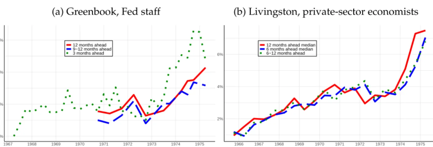
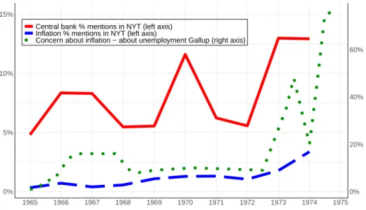
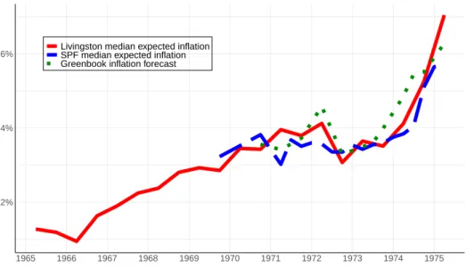
The data are consistent with the narrative analysis of the Fed's statements in the previous section that held that the successive spikes in inflation were one-off temporary blips. Inflation is almost always expected to be higher in the near term than in the longer term. Moreover, signs that the anchor was moving in a quantitatively significant manner only appeared in the early 1970s.
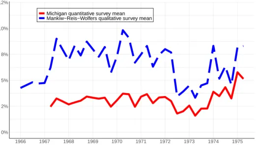
Again, there is no observable trend in the central tendency of the household survey until the end of the decade. However, the literature that has focused on the last 40 years also shows that the cross-sectional distribution of expectations contains much more information (Mankiw, Reis and Wolfers, 2004, Coibion and Gorodnichenko, 2012). Beginning with the 1968 projections of inflation in 1969, the disagreement in the series begins to increase markedly for about two years.
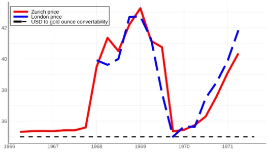
Then, between 1971 and mid-1973, incomes policies seem to have worked as Burns supposed, reversing the rise in expected inflation. The relative decline in 1972 and the upward rise after the oil price shock follow the patterns of disagreement in the household survey. Finally, the gold price in USD, which traded freely on the London Mercantile Exchange, is not a reliable indicator.
The market grew in activity during the gold pool in the London market, trading in multiple currencies. Already between 1967 and 1970 the anchor forced as revealed by market prices for gold futures, public concern and media reports and, perhaps more convincingly, by the shift in the cross-sectional distribution of household expectations.
4 A measure of fundamental expected inflation
A model
The first equation suggests that the inflation expectations reported by household h in the survey follow an exponentially modified Gaussian (EMG) distribution Ft(.), the sum of three parts: the first part is just the prior meanπ∗t of what the underlying expected inflationπte might be. It is important to consider the fact that expected inflation in the survey is persistently above actual inflation, perhaps as a long scar from the high inflation of the 1970s and 1980s. The third is an individual-specific baseline signal with noise eth derived from a normal distribution.
Reis (2021) shows that this model captures key properties from the large literature on imperfect information, overreaction, experiential learning, and contagion. The second equation states that expected market price inflation qt is equal to expected risk-adjusted inflation with risk adjustment y(πet). This expectation is formed by traders who start from a money that is EMGFt (.) (traders are human after all), but which is updated according to Bayes' rule after observing the market price itself, as written in the second equation.
The third equation states that survey professionals are similar to inflation risk traders. They use Bayes' rule to combine the information that households have with market prices, but what they report in a survey is neither risk-adjusted nor does it identify who is the marginal player in the markets. Rather, from the small samples in these surveys we can only see the objective beliefs of the average trader.
The information in different data, and the model to filter it
To bring the model to the 1966-71 annual sample, I use the three moments from the Michigan Quantitative Survey, the mean expectation of the subset of professionals in the Livingston study who work in the financial industry, and the annual expected inflation implied in Zurich gold futures. As of 1972, there is no clear market price to implement the model. Following Reis (2021), I equate it to 2, which creates a significant amount of noise in the financial markets.
First, the data on market prices comes from the Zurich Gold Market, but the data on survey of market participants comes from professional economists in the United States. Second, there is no data with which to calibrate changes in the inflation risk premium, so I assume it is constant (and since the model only identifies changes, I set it to zero: y(πe) = πe). For short-horizon expectations, the different structural models of expectations in the literature are too diverse to be captured in a parsimonious way.
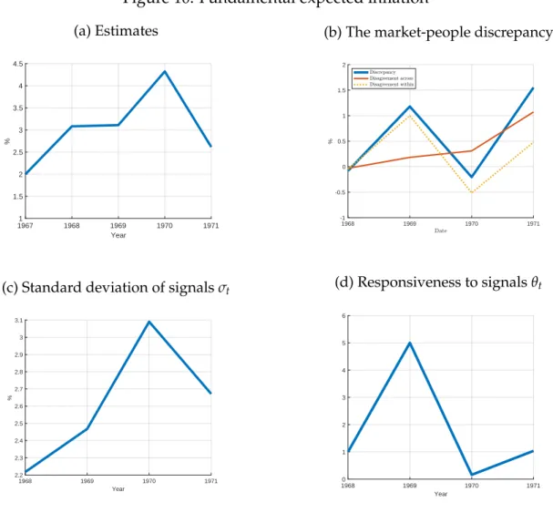
The estimates of fundamental expected inflation
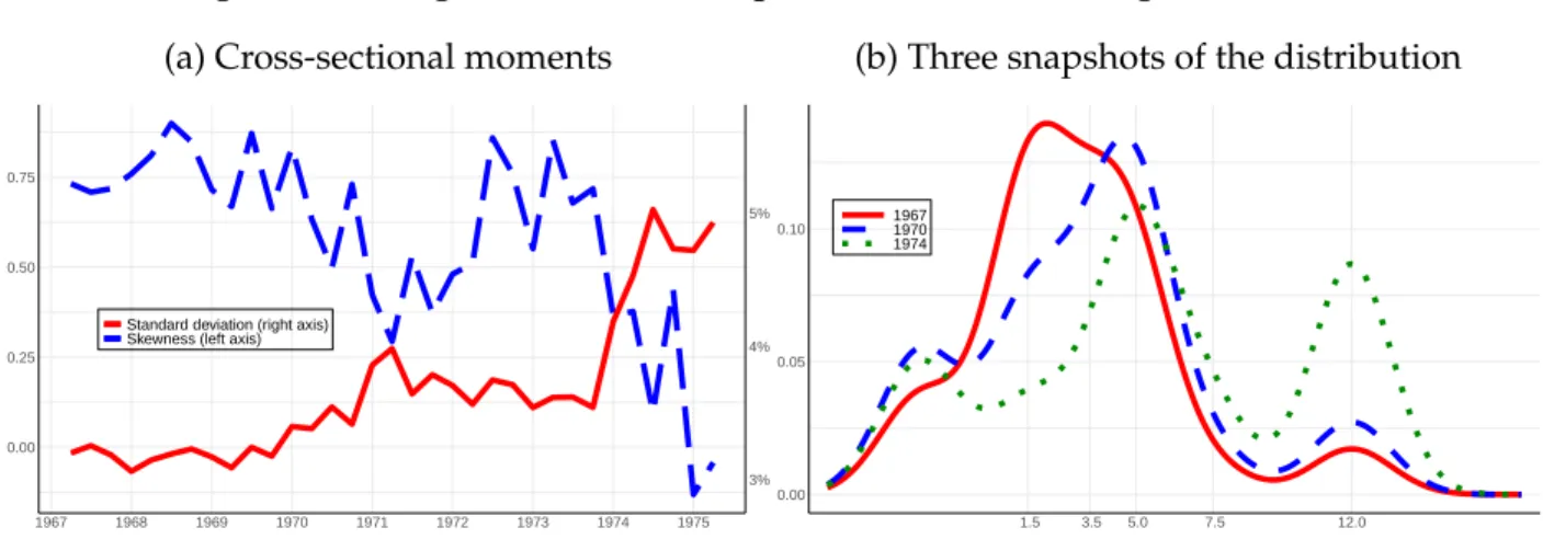
Instead, the rising market prices, combined with the large increase in the standard deviation and the decrease in skewness across households, reveal that fundamental expected inflation changed significantly. However, due to the increase in variance and decrease in skewness, the model places considerable emphasis on this being instead a result of an expected increase in inflation. In 1970, the rise in survey expectations combined with the movements in the disagreement confirm that the fundamental has increased, so the model updates its estimate further up, even though market prices have fallen.
Panels (c) and (d) show the time series of two important model parameters, σt, which measures the distribution of idiosyncratic signals, and θt, which measures how much an individual will respond to his or her individual signal. If people were pure Bayesians, then θt would be proportional to the inverse of σt, but the model allowed this not to be the case following theories of overconfidence, overreaction, and diagnostic expectations. But at first they are also more responsive to their individual signals, as if they are paying more attention to the path of inflation.
5 Measuring the expected inflation anchor in other episodes
- Brazil, 2011-16
- South Africa: 2010-2016
- The United States in the 1980s: dropping the anchor
- United States 2020-21: Where is it heading?
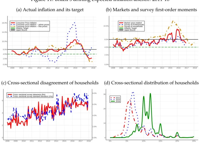
Rather, the first moment of the household survey begins to take off clearly from the beginning of 2013. The increase in variance and skewness clearly results from a subset of households breaking off to the right of the median. Third, that measures of disagreement in the cross-sectional survey provide a good picture of the loss of the inflation anchor, but one should not expect them to be captured by a naive time series correlation between standard deviation and skewness.
The initial shift in the US anchor came with a thinning of the left tail of the distribution: those who expected very low inflation joined the median. The loss of the inflationary anchor can come quickly and not necessarily build up gradually, as happened in the US in the late 1960s. First, the rise in global oil and commodity prices in 2010-2012 pushed inflation towards the upper end of the range.
By 2015, these effects wore off and inflation fell sharply to the middle of the target range, leading the SARB to ease monetary policy. Again, headline inflation moved to the upper bound of the target, although core inflation was within it, and again the SARB kept monetary policy steady. 20 For a description of the SARB's response to successive shocks, see Kabundi, Schaling and Some (2015) or Mminele (2019).
Between the start of 2020 and the second half of the year, mass moved away from the top of the bell-shaped distribution and towards the right tail. Perhaps, as in the early 1980s, households are ahead of the curve in detecting a change in regime.
6 Conclusion
In the first half of 2021, it was rather the left tail that was hollowed out. Or, perhaps through the overconfidence discussed in the model, a few price changes in key goods overinfluenced overall inflation expectations, much like the wage and price controls in the US in the 1970s, the administered prices in Brazil in the 2010s, and the food and electricity prices in South Africa in the 2010s. factors.
This article adds a new element to the poor measurement class of Great Inflation explanations: the poor measurement of inflation expectations. These errors compounded each other by missing the drift of expected inflation and thus failing to prevent its loss. The rise in the most notable price of gas caused low inflation expectations to rise rapidly and by leaps and bounds.
The paper confirmed the usefulness of using data on inflation expectations and showed that:. i) they also detected the loss of the inflation anchor in Brazil in 2011-2016; (ii) even if Turkey did not have a very strong anchor and the events are still too young to be sure, the expectations data indicate a significant change in 2018, (iii) the expectations data do not produce false positives in South Africa 2010-2016, but show a stable anchor of expectations despite many negative shocks to actual inflation, and (iv) they move consistently even when the anchor goes out to sea. bed as in USA 1979-84. Looking at current events, the data suggests that the anchor has moved in 2021, but it's still early enough that good politics or luck can keep it in place for the foreseeable future. Much work remains to be done in the future to provide better measurements of the expected inflation anchor.
Knotek, Edward S., Raphael Schoenle, Alexander Dietrich, Keith Kuester, Gernot M¨uller, Kristian Myrseth, and Michael Weber. To understand the core drivers of inflation in South Africa." Keynote speech at SP Dow Jones Indices South African seminar.