To my colleagues and friends of the MEGT 1998 course, I am also very indebted for the times we spent together. Of the assumptions of this model, two of them can significantly limit its application in more complex industrial processes.
Summary of Contributions
We also aim to define alternative production strategies, which are ultimately more suitable for different business environments. ii) The use of the Infinitesimal Perturbation Analysis methodology to find the optimal parameters of the pre-defined strategies, which has shown to be a technique with great potential. iii).
Organization of the Thesis
Appendix C – The SimulGlass package, provides a cd-rom with a ready-to-install version of the software package and an Acrobat file with the full version of the thesis. However, single product models are able to simulate the main features of the larger problems.
Single Product, Single and Multiple-Stages Models
The cost variable can be broken down as follows: averaging versus discounting – when the time value of money is an important issue, the discount rate must be considered; Order cost structure - the simplest assumption is to consider costs proportional to the number of items required. Conversely, if the initial inventory x is below the level of s, the optimal decision is to order to S.
Multi-Product, Multi-Stage Models
Operations Research Perspective
These results usually refer to non-optimal base stock variant policies, proposed as heuristics for finding variables to decide on sub-optimal problems. Third, the CW base inventory level appears insensitive to the number of retail outlets, suggesting that retailers with unequal levels of demand would behave similarly.
Control Theory Perspective
Finally, the general behavior of the optimal inventory policy does not seem to be sensitive to the service criterion. This work is important because there are any number of machine states that correspond to different failure states in the system.
Make-to-Stock vs. Make-to-Order
Modeling Issues
When a machine switches from producing one part to another, the machine's configuration must be physically changed. Some authors consider labor as a single resource and assume that all levels of labor can be accommodated within the factory.
Random Yield
Modeling of Yield
A second way to model yield uncertainty is to define the distribution of the fraction of good units, often referred to as rate of return or stochastically proportional return. The third modeling approach considers that the distribution of the fraction of good items changes with the batch size.
Production Decisions in the presence of Random Yield
In such systems, the output quantity is the minimum of the input quantity and the available capacity. Moreover, the amount to order depends not only on the expected random return, but also on the second moment of the random return.
Infinitesimal Perturbation Analysis
The Key Features of Perturbation Analysis
In a manufacturing system, for example, we may be interested in the effect of changing the processing time of one machine on the overall throughput of the system. On the other hand, if we use PA, the gradients of N can be determined from a single simulation.
Finite and Infinitesimal Perturbations
Consequently, the main limitations of infinitesimal perturbation analysis are related to the incorporation of such a technique into a general simulation language.
Perturbation Generation and Propagation
The framework used is a periodic review, capacity, multi-product, production-inventory system operating under a level base stock policy. To be precise, given a particular product p and stage s, it is necessary to add all the downstream inventory from that stage to calculate the scale inventory. In the framework of discrete-time inventory control, the problem addressed now analyzes several different production policies, which are tested in perfect and random yield production systems.
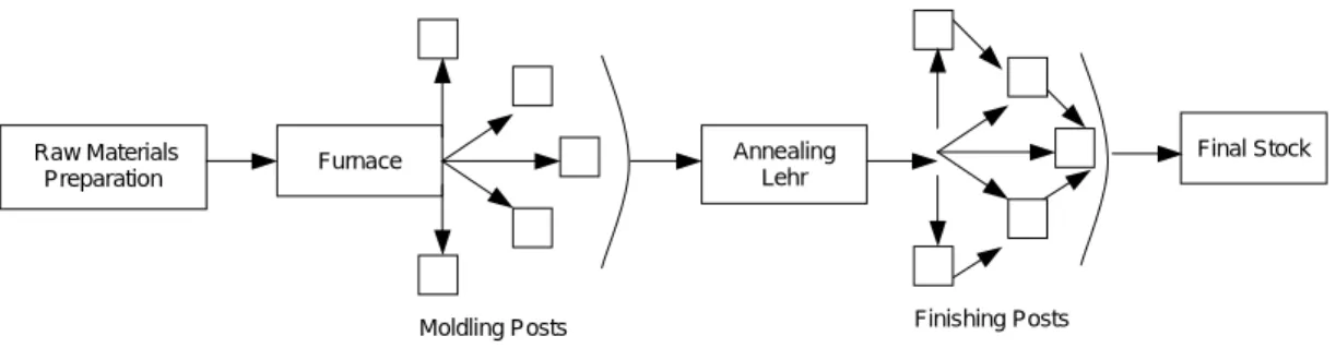
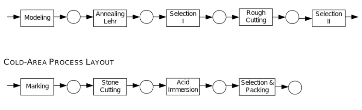
The Glass Manufacturing Process
As far as the capacities of the furnace, the casting pillars and the roaster are concerned, they are all finite. After being extracted from the final stage of the hot zone, most items must go through a series of finishing processes (marking, stone cutting, acid dipping, and sorting and packaging). The capacity of the posts is limited and the setup times of the various posts are negligible when compared to the processing time of the operation.
Production Strategies
That is, an MTO strategy is an MTS strategy with the Z levels set to zero. To reduce product production time, an intermediate stock of products with the same basic geometry can be created. In other words, a DD policy is an MTS strategy with cold zone Z levels set to zero.
The Basic Model
- Variable Classes
- The Performance Measures
- The Derivatives of the Basic Model
- State Variables Derivatives
- Performance Measures Derivatives
Echelon base stock, production limit, and capacity variable form a class of control variables. The most common criteria are: .. i) level of service type 1 – the proportion of periods in which the entire demand is met; .. ii) Level of Service Type 2 – Proportion of demand that is immediately satisfied by inventory. Additionally, and within the scope of this thesis, we will deal with an indicator that expresses the time delay from the moment the client's order arrives to the moment the entire order is delivered - flow time.
The Production Decisions and their Derivatives
The Production Decisions Algorithm
While in the above the ordering is based on an absolute value of the shortage, here it will be based on a weighted shortage, i.e. the absolute value of the shortage divided by the average demand. In [Bispo, 1997], section 3.4, the production decisions are determined to continuously compensate for any product shortage. For the product with the higher weighted shortage, the production decision is the shortage value if there is available capacity, upstream inventory and if the production limit is not exceeded.
Infinitesimal Perturbation Analysis Validation
System and Products Data
Cost Structure
As described in section 3.2.4, the developed cost structure takes into account three important direct costs: raw material costs, energy costs and direct labor costs. The following table shows the values of energy costs and labor costs for all process phases. A factor of 1.3 is used for high demand products, 1.4 for medium demand products and 1.5 for low demand products.
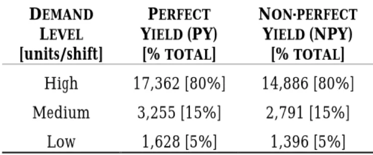
Demand and Yield Structures
The yield factors used in the numerical experiments are the same as those available in the company's information system and obtained from historical data. The forming stage has the lowest average yield, partly explained by a strong dependence on human labor and the degree of complexity of the operation. It should be mentioned that the application is not limited to considering phase-dependent yield factors.
Simulation Cycles
Numerical Results
- Numerical Results Confidence Interval
- Limited Production Approach (LP)
- Non-Limited Production Approach (NLP)
- Discussion on Optimal Convergence
- Weighted Shortfall versus Non-weighted Shortfall
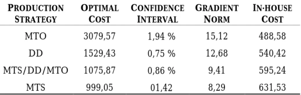
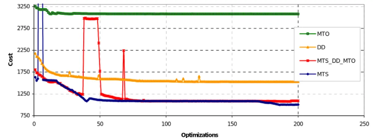
If we introduce production randomness (see Table 4.3 for yield factors), we are now interested in comparing the performance of the system with scenario 1. Despite the non-convergence to the optimal values, we are confident that the obtained qualitative behavior will not change with slightly more accurate results (see Figure 4.6 and Table 4.16 for such a case). Take for example “Optimization B (LP-NPY)” from Table 4.16, where the norm of the finite gradient is slightly less than 3, in an optimization problem with 306 variables.
Hardware and Time Requirements
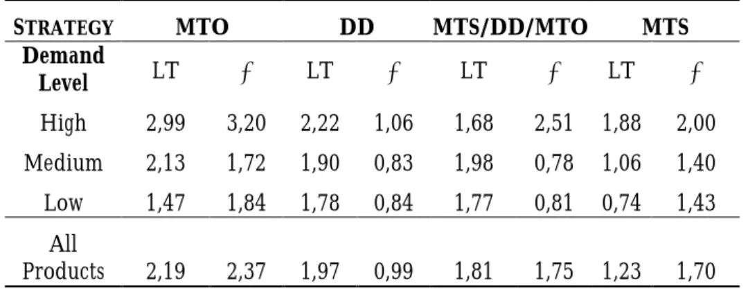
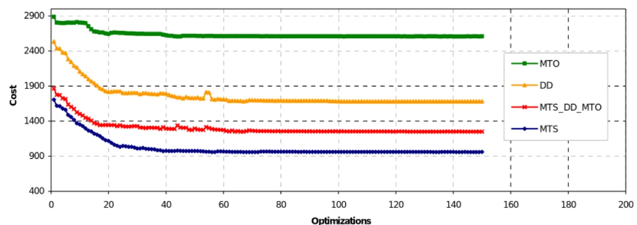
The implications of the results presented in this chapter in terms of defining the most appropriate strategy will be discussed in Chapter 5. A set of computational experiments is presented to gain some insights into the impact of the different production strategies on the performance measures. The numerical results from the previous chapter clearly show that a make-to-order strategy incurs fewer internal costs than all the other strategies, while at the same time having the highest average total costs and the worst lead times.
Future Research
Then, implementing and comparing the performance of alternative optimization algorithms would be a further step to improve the quality of the generated results. OPTIMAL – Calculates the optimal values of the decision variables Z and U, according to the production strategy defined by the user;. As can be seen in Figure B.2 (see Appendix B), the Product Parameters window has three tabs, each for different product groups (divided by demand level - High Demand Products, Medium Demand Products and products with low demand), in which the information about the products should be entered, as shown in table A.1.
System Cost Structure Window
The Default Values button enables quick entry of all default data related to the product parameters present in the DATA module. The Default Values button, shown in Figure B.3, allows you to quickly insert all the default information contained in the DATA module and related to process costs. This set of numbers will be used, as discussed in Section 4.2.1, to determine the product holding costs hps and penalty costs bps used to determine the total costs associated with a given production strategy.
Decision Variables Window
Selecting the All Products DD button runs the application simulating all products under a delayed differentiation policy. Box Selection of one of the available policies for each product p All products MTS button Selection of Make-to-Stock policy for all products All products MTO button Selection of Make-to-Order policy for all products. All products DD button Selection of delayed differentiation policy for all products MTS/DD/MTO button Selection of a combined policy according to the demand level (high demand – MTS, medium demand – DD, low demand – MTO).
Simulation and Optimization Parameters Window
During the execution of the program, its evolution can be verified on the two available counters: the Simulation counter and the Optimization counter. Optimizations Maximum number of optimization iterations Phases Capacity Definition of the capacity of each process phase [min.]. Choice between raking or not, the shortage weighted with the average demand for production decisions Algorithm Simulations Counter Number of simulations already completed Optimizations Counter Number of optimizations already completed.
The SimulGLASS Output
Historical Cost and Optimal Z and U Values
Minimum step Minimum step value to guarantee convergence Epsilon Minimum cost difference to guarantee convergence Epsilon D Minimum value to guarantee the condition of Stability. Counters Switch Toggles the counters Run button ON and OFF Starts the Simulation/Optimization process Main Menu button Returns to the application's Main Menu .. generated automatically by the application. Basic stock levels Z* and production limits U*, for all products at each stage s, corresponding to the system's minimum cost scenario – the so-called optimal values; .. iv) The gradient of the cost function and its rate, which corresponds to the minimum state of the cost of the process;
The Lead-Times
The Simulation Module
- Demand and Yield Generation Procedure
- Echelon Update Procedure
- Shortfall Update Procedure
- Production Decisions Procedure
- Inventory Update Procedure
- Cost Update Procedure
- Lead-Time Procedure
Once the grade stocks are calculated, it is possible to estimate the amount needed to reset the base stock level - the deficit. To sort the weighted deficit matrices, two sorting algorithms were implemented—selective sort (n2 rank) and quick sort (n.log(n) rank) as presented in [Cormen et al., 1997]. Such an update is performed according to equations (3.1) and. 3.16–17), which correspond to inventory variables and inventory derivatives, in that order.

The Optimization Module
The Fletcher and Reeves Algorithm
As described in [Bazaraa and Shetty, 1979], Fletcher and Reeves' conjugate gradient method deflects the direction of steepest descent by adding a positive multiple of the direction used in the last step. By successively reducing the step size, let xi+1 be the first value that leads to a success for xi, always using direction di.
Testing the Software
To install, simply insert the CD-ROM into the drive, click the setup.exe file, and follow the installation instructions. A full version of this thesis is also available on the CD-ROM (see the file MasterThesis.pdf). Thesis, Graduate School of Industrial Administration and the Robotics Institute, Carnegie Mellon University, Pittsburgh, PA.