Modelling, Simulation, Analysis and Stabilization of a ... - Fenix

Condição de equilíbrio e funções de linearização são desenvolvidas como forma de obter e analisar versões linearizadas do modelo não linear. As funções para condições de equilíbrio e linearização são validadas comparando as respostas dos modelos lineares e não lineares.

Abstract

Nomenclature

Introduction

Motivation
Objectives
Main Contributions
Thesis Outline

Investigate how search methods can be implemented to obtain trim conditions for the non-linear model of the aircraft. The last section shows a representation of the simulator implementation together with the complete model of the aircraft.

Vehicle Dynamics Model

Atmosphere Model
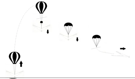
The Flying Wing Vehicle
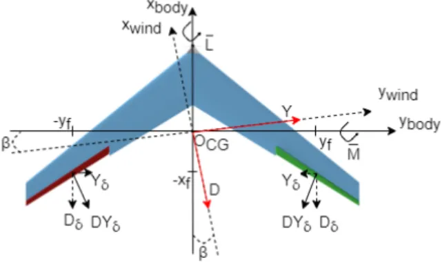
Reference Frames
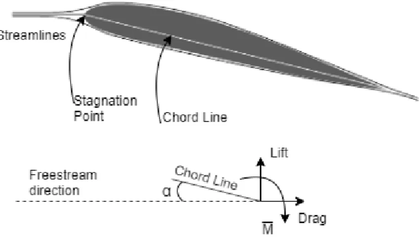
Aerodynamics
Propulsion
Dynamics Equations
Kinematics Equations
Flying Wing Simulator

In aeronautics, it is practical to define a frame of reference for the wind axes, since the aerodynamic forces and moments on the aircraft are the result of the movement of the body relative to the air, and these effects depend on the orientation of the aircraft relative to the air flow. For this type of work, an understanding of aerodynamic expressions and mathematical models that contain complete aerodynamic data for an aircraft is mandatory. The remaining expressions related to the angular velocities are also available from the aerodynamic analysis of the wing [5] and are normalized to radians as they are usually in rad/s.

For the drag, lift, and pitching coefficients, the sum of the flap lift forces depends on the direction of the flap deflections, since lift is a force perpendicular to the freestream that models the elevator effect. The flap roll coefficient is obtained as a projection of the flap lift on the y-axis relative to the lateral center of gravity. Similarly, the flap slope coefficient is obtained as a projection of the flap lift force on the x-axis in relation to the longitudinal center of gravity.

The drag contribution to this effect is the projection of the collision drag force on the y-axis, while the lateral collision force contribution is the lateral collision force projected onto the x-axis, relative to the center of gravity. First, the gravitational force Fg ensures that the weight of the aircraft is taken into account, rotating from the reference frame NED to the reference frame ABC (equation 2.65).

Flying Wing Model Characterization

Flight Envelope
Aircraft Trimming
Linearization
Longitudinal Model Analysis
Lateral Model Analysis

As for the maximum speed limit, some approximations can be made to determine this limit. When analyzing these equations, it can be seen that altitude plays an important role in determining the envelope of the aircraft's flight speed. As for the upper flight limit, the maximum altitude should be defined as the limit where the aircraft begins to lose maneuverability (the case where the flap deflections or the propulsion system fail due to thin air).

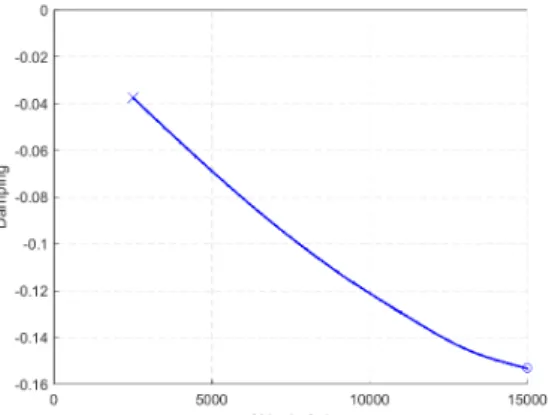
In the case of motorization, the rate of climb γ can be imposed, since in the case of gliding flight γ is a result of the algorithm. As for the climb angle, this variable will be given as a result of the trimming process by the algorithm. As for the variation in air speed, it is difficult to make assumptions as it has a small influence on the short-period damping.

Varying the altitude and airspeed for the lateral model, without motorization, results in the pole evolution shown in Figure 3.8, which reveals the expected lateral mode poles. For the case where motorization is used, the pole evolution is shown in Figures 3.10, which shows that the poles are similar to the case without motorization, as previously seen for the longitudinal model example.

Control Design

Controllability
Classic Control
Optimal Control
Linear Control Simulator Implementation

Given that the structure of these arrays does not change radically with altitude, airspeed, or with glider-powered flight, this example will serve as a demonstration of the controllability of the flight envelope. The proposed control method for the non-motorized longitudinal model (Figure 4.1) is pitch feedback with a PI-D controller and inner loop feedback for pitch rate (pitch damper effect). A negative unity gain was used for the damper as this simple value provides better damping for the short-period complex pair as shown in Figure 4.2 where flight conditions of 2500m altitude and 20m/s airspeed were used.

The proposed control method for the lateral model (Figure 4.3) is a roll feedback with a PI controller for steady-state improvement with an internal loop feedback for the roll speed (roll damper). The gain for the damper was used as positive unitary gain, because this simple value guarantees a stabilization of the dutch-roll complex pair, as shown in Figure 4.4. The use of an LQR achieves the optimal state variable feedback control through the minimization of the performance index Jc, where matricesQ and R are the relative importance of the error for the considered states and the energy consumption for the considered inputs, respectively.

Using thematlabcommandLQR, the resulting matrix is 2x4, and since there are only two actuator inputs available, it is desirable to only request values for forward speed and pitch angle. The gain matrix will be split into a gain matrix for the demand Kreq in the outer loop, and a gain matrix for the state regulation Kreq in the inner controller loop.

Results

Trimming Results

Looking at all the results for powered flight, the importance of aileron deflection resolution (Figures 5.3(f), 5.4(f), 5.5(f) and 5.6(f)) is significant as the proposed values for this variable are considerable. small, which means that very small differences in the elevon system have a large effect on lateral stability. This detail is important for the physical implementation of the aircraft, as the servo motors responsible for flap deflection must provide high resolution for individual deflection angles. The input values used for the climb angle results were from -5 to 5 degrees in 2.5 degree increments (Figures 5.3(d), 5.4(d), 5.5(d), 5.6(d) and 5.7(d) ) and shows the common sense result that the upper flight limit decreases with increasing climb angle.

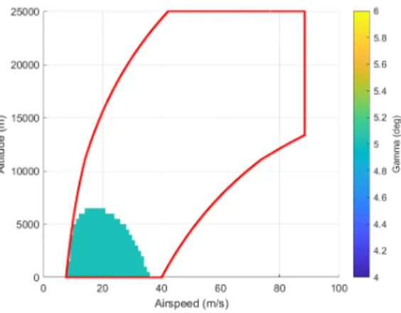
These results are not considered as they may be a way to set the lower climb angle limit, as descent at high airspeed may represent a dangerous maneuver for the aircraft. This can lead to the interpretation that wider blue areas enable a greater variety of use of the car in battery saving conditions. To consolidate these results, a map of the flight envelope is presented below on figure 5.1 detailing the given regions where the aircraft can glide or impose a climb angle (with limits from -2.5 to 5 degrees).

In a final note on the trim results, it should be noted that the a values never reach the theoretical stall limit as they are more conservative. This is probably a consequence of the effect of the lift coefficient of the flaps and the non-linearity from the attitude effect on the gravity vector, which was neglected in the estimation of the stall speed.

Control Results

Regarding the flight decks for powered flight, the results obtained from the reduction process for different values of γ have always considered that the control surfaces must retain an additional maneuverability. This effect has not been modeled theoretically, but it can be interpreted that the flight ceiling is a consequence of air thinning, meaning that the propulsive and aerodynamic forces have insufficient air surrounding the aircraft to maintain balance. This is probably a consequence of the effect of the flap lift coefficient and the non-linearity from the attitude effect on the gravity force vector, which are neglected for the stall speed estimation. a) Flight canopy for gliding flight.

Flight envelope map showing the different areas of maneuverability. for the cases where the lower air speed of 20 m/s is taken into account. The gains obtained for these PI-D controllers are specified in Tables 5.1 and 5.2, where the lateral model has additional values for the 10 km altitude, as this is the high altitude within the flight range used to study the powered flight. While the response has stabilized, the requests only work when made individually, and still. a) Cost function evaluation over the flight range. b)αvariation across the flight envelope. c)δvariation across the flight envelope. d)γvariation over the flight range.

Comparison of the linear and nonlinear responses, even for the non-required variables, shows further evidence of well-preserved dynamics by the linearization process. The gains for each point on the flight envelope, shown in Table 5.3, are varied through the LQR command which means that a gain planning system must be implemented for each change in altitude and airspeed. The performance of the PI-D controller for the lateral model is satisfactory for the settling time and overshoot requirements, although it cannot remove the oscillatory component from the Dutch rotation. a) Estimation of the cost function over the flight envelope. b) αvariation over the flight envelope. c) variation on the flight envelope. d) γvariation over the flight envelope. e) δvariation on the flight envelope. f) variation on the flight envelope.

The gains are affected by variations in altitude and airspeed, so this PI-D controller requires a gain planning method over the flight area. a) Cost function evaluation over the flight envelope. b)α variation over the flight envelope. c)δ deviation over the flight envelope. d)γvariation over the flight envelope. e)δthvariation over the flight envelope. f)δavariation over the flight envelope. a) Cost function evaluation over the flight envelope. b)α variation over the flight envelope. c)δ deviation over the flight envelope. d)γvariation over the flight envelope. e)δthvariation over the flight envelope. f)δavariation over the flight envelope.

Conclusions

Achievements

The search method only requires a definition of the nonlinear model, the chosen free variables, a starting point for the free variables and a set of constraints. Most of the results obtained regarding the pruning algorithm were consistent and the solutions were continuous. These tools allowed the flight envelope for this aircraft to be defined for gliding and powered flights, which will be useful to study the viability of the HABAIR concept, revealing many characteristics of the aircraft.

The set of equilibrium points resulting from the trim functions allows the derivation of a linear model, showing the decoupling between the longitudinal and lateral variables. As for the controller, two methods were achieved using classical and optimal control techniques, which produced satisfactory results. One method involves the PI-D controller, for the longitudinal model with pitch feedback via the elevator deflection and a pitch damper, while the lateral model was controlled by a PI-D controller with roll feedback via the aileron deflection and a pitch damper. .

Both control techniques allow validating the linearization function as a tool to derive the longitudinal and lateral models, while preserving the key dynamics of the nonlinear model. It can then be concluded that the flying wing vehicle is a valid option for the HABAIR concept.

Future Work

Bibliography