The two-period monetary economy under flexible prices
Introduction
In order to stick to simplicity and focus on innovations in monetary balance, we abstract from investment decisions and consumption and leisure choices. In what follows, we assume that prices are flexible in order to focus on long-run issues. In Section 4, we describe the equilibrium in the goods and services market and in the money market.
In Chapter 5, we analyze how the main variables of the model adjust to temporary, permanent, and expected changes in the money supply or actual disturbances.
Nominal and real budget constraints
- The household budget constraint
- The interest rate parity condition
- The government budget constraint
- The Fisher parity condition
- The real interest rate parity
- Real budget constraints
This means that the return on foreign bonds, in addition to the interest payment, may include a capital gain or a capital loss related to exchange rate fluctuations. In the absence of restrictions on capital movements, the household will choose the currency composition of the portfolio to maximize the value of its lifetime wealth. The proportional change in the price level between period 0 and period 1 is the current inflation rate, 1P P1 01.
As can be seen from the appendix, in a context of uncertainty there will be an additional term that conveys the nominal and real interest rates related to the risk premium. This equation shows that the accumulation of real money balances plays the same role as taxes in the budget constraint. Money and taxes do not appear in the economy's intertemporal budget constraint: they only redistribute income between domestic agents4.
Optimal consumption and money demand
- The household problem
- Money demands
- Optimal consumption
The real money demand (28) is a positive function of private consumption, which captures the transaction demand for money, and a negative function of the nominal interest rate, which is the opportunity cost of holding money. This reward is the nominal interest rate, which serves as the opportunity cost of holding money. The demand for money in period 2 (29) is purely "classical", in the sense that it only accounts for the transaction motive.
Therefore, the demand for money (29) can be interpreted as a limiting case of equation (28) with the opportunity cost of holding money to infinity.
Equilibrium
- Equilibrium in the market for goods and services
- Equilibrium in the money market
- The pieces together
The nominal interest rate opens a channel through which expectations of future central bank actions affect the price level today. This equation states that the nominal interest rate is determined by the time course of the money supply from periods 1 and 2. The demand for money (28) is described by a negative relationship between the quantity of real money and the nominal interest rate.
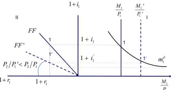
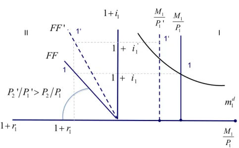
The central bank sets a certain path for the amount of money today and in the future by determining the nominal interest rate. Based on the nominal interest rate and consumption today, the demand for real money is determined. Mediating the nominal interest rate and the real interest rate is the Fisher equation (12), described by the FF schedule in panel II.
The FF schedule shows a positive relationship between the nominal interest rate and the real interest rate. In the infinite horizon case, the interest rate in period 2 depends on the money supply in period 3, and the interest rate in period 3 depends on the money supply in period 4, and so on. This means that the entire path of future money matters in determining the interest rate today.
In view of (37b), the current period's nominal interest rate deviates from the steady interest rate, i2, depending on how far the rate of money growth between period 1 and. Compared to (37), we see that this formula is more realistic for calibration purposes, as it does not imply nominal interest rate around 100% when the money supply is constant over time.

Comparative statics
- Permanent monetary expansion
- Anticipated monetary expansion
- Temporary monetary expansion
- Temporary output expansion
- The classical dichotomy
Since the disruptions occur on the monetary side of the economy, the real side will not be affected. On the other hand, today's price growth has lowered the real value of the country's initial debt. These two effects together mean an increase in the price level (and until then a nominal depreciation of the exchange rate), but less than in proportion to money.
In the limit, even if the nominal money supply expanded to infinity, the nominal interest rate could not fall below zero. As we know, the real interest rate is determined under flexible prices in the real side of the economy. In the open economy case, the real interest rate remains unchanged, and the current account turns into a surplus (point 1').
In the case of a closed economy, the real interest rate falls so much that current consumption corresponds to the new level of production (point 1''). Therefore, private consumption and money demand increase more in period 1 than in the case of an open economy. In an open economy, the real interest rate remains unchanged, so the slope of the FF curve cannot change (point 1' in Panel III).
The reason is that the price level in period 2 and period 1 decreases in the same proportion, leaving expected inflation unchanged. In the case of a closed economy, the current price level decreases, but the future price level remains unchanged, so the FF curve must shift upward giving the same nominal interest rate despite the fall in the real interest rate (point 1' ' in panel II).
Fiscal aspects of money
- The key role of expectations
- Credibility and fiscal sustainability
- Inflation: monetary or fiscal?
Credibility can only be gained if the Treasury is willing to adjust the level of taxation to cover the funding gaps implied by changes in the money supply. If the government cannot commit in advance to raising taxes in the future to pay for these bonds, remote agents will predict that the government will end up printing more money, generating more inflation today. In the analysis of monetary shocks above, we have abstracted from the sustainability of government finances, assuming that changes in monetary policy are matched by changes in taxation.
The authors' main proposition is that in the absence of fiscal adjustment, any central bank effort to reduce inflation today will come at the cost of higher inflation in the future6. Suppose the central bank wanted to lower the current rate of inflation (11 P P1 0 ) by lowering the price level today. However, the government does not intend to implement any fiscal adjustment today and cannot commit to a fiscal adjustment in the future.
In that case, forward-looking agents will perceive that the only way for the government to cover the financing gap resulting from lower foreign exchange earnings today will be to expand money in the future. To see this, note that while the temporary monetary contraction in Figure 6 causes the current price level to fall relative to the base case, the expected monetary expansion (Figure 5) causes the current price level to rise: intuitively, the additional increase in the rate of interest supplied by future money expansion causes the demand for money to fall today, and at that time an increase in the current price level. Formally, the key parameter is the elasticity of the demand for money in relation to the interest rate: the more the demand for money reacts to the additional increase in the interest rate (in figure 5), the more likely the possibility of the net effect. to be an increase in the current price level, contrary to the monetary decline.
As you can see in the numerical exercises at the end of this handout, a monetary contraction in period 1 with such a functional form, followed by a budget-neutral monetary expansion in period 2, leaves the current price exactly unchanged. If the government cannot credibly commit to raising taxes in the future to meet the government's intertemporal budget constraints, foresight agents will anticipate further money pressures.
Summary
Let Bt* be the amount of foreign bonds backed by a foreign exchange forward contract, and Bt* be the amount invested in foreign bonds that are unsecured. For simplicity, we assume that no bonds are held in period 0 and that the household pays no taxes. If the household is risk neutral, the marginal utility of consumption is constant in period 2 and the risk premium disappears.
The nominal interest rate adjusts to inflation in the light of equation (a7), and at that time the demand for money is indirectly affected, but there is no direct effect of inflation or of uncertainty about inflation on the demand for money. Similarly, there is no other asset return that affects the demand for money: changes in the foreign interest rate or in the real. The government does not consume, so the lifetime income from foreign exchange earnings is transferred back to households in period 1. The government budget constraint is given by .. a) From the consumer optimization problem, find: (a1) the optimal consumption in period 1; (a2) the optimal demand for money in periods 1 and 2. b) Find the expression for aggregate supply and national expenditure in this economy and find the autarky real interest rate.
Assuming (c), suppose the Treasury decides to expand the money supply to M1 400 in the first period. Find out the implications of this policy on (d1) the nominal interest rate in period 1; (d2) the price levels in period 2 and in period 1; (d3) the real money supply in period 1. The required increase in taxes (b4) Describe the initial equilibrium in a graph. c) Assuming (b), instead assume that government taxes did not increase in period 1.
In that case, (c1) how much must M2 increase to offset the fall in the current money supply to M1 300. The government does not consume, so any income from revenue money will be transferred back to the household in period 2. In that case, how much will be: (c1) the nominal interest rate. c4) the transfer to households in period 1. c5) Describe the adjustment in light of the 3-panel graph.
Find: (a1) expressions for aggregate supply and expenditure; (a2) current account; (a3) nominal interest rate in period 1; (a4) price levels in period 2 and period 1; (a5) real money supply in period 1; (a6) Describe the initial equilibrium on the 3-panel graph.
Money demands and parity conditions in a context of uncertainty 33