Preface to the Instructor’s Manual

(1)

Volume 2: Presentation Material

Behrooz Parhami

Department of Electrical and Computer Engineering University of California

Santa Barbara, CA 93106-9560, USA E-mail: [email protected]

© Oxford University Press, Fall 2001

(2)

This instructor’s manual is for

Computer Arithmetic: Algorithms and Hardware Designs, by Behrooz Parhami ISBN 0-19-512583-5, QA76.9.C62P37

For information and errata, see http://www.ece.ucsb.edu/Faculty/Parhami/text_comp_arit.htm All rights reserved for the author. No part of this instructor’s manual may be reproduced, stored in a retrieval system, or transmitted in any form or by any means, electronic, mechanical,

photocopying, recording, or otherwise, without written permission. Contact the author at:

ECE Dept., Univ. of California, Santa Barbara, CA 93106-9560, USA ( [email protected] )

(3)

Preface to the Instructor’s Manual

This instructor’s manual consists of two volumes. Volume 1 presents solutions to selected problems and includes additional problems (many with solutions) that did not make the cut for inclusion in the text Computer Arithmetic: Algorithms and Hardware Designs (Oxford University Press, 2000) or that were designed after the book went to print. Volume 2 contains enlarged versions of the figures and tables in the text as well as additional material, presented in a format that is suitable for use as transparency masters.

The fall 2001 edition Volume 1, which consists of the following parts, is available to qualified instructors through the publisher:

Volume 1 Part I Selected solutions and additional problems Part II Question bank, assignments, and projects

The fall 2001 edition of Volume 2, which consists of the following parts, is available as a large file in postscript format through the book’s Web page:

Volume 2 Parts I-VII Lecture slides and other presentation material

The book’s Web page, given below, also contains an errata and a host of other material (please note the upper-case “F” and “P” and the underscore symbol after “text” and “comp”:

http://www.ece.ucsb.edu/Faculty/Parhami/text_comp_arit.htm

The author would appreciate the reporting of any error in the textbook or in this manual, suggestions for additional problems, alternate solutions to solved problems, solutions to other problems, and sharing of teaching experiences. Please e-mail your comments to

[email protected]

or send them by regular mail to the author’s postal address:

Department of Electrical and Computer Engineering University of California

Santa Barbara, CA 93106-9560, USA

Contributions will be acknowledged to the extent possible.

Behrooz Parhami

Santa Barbara, Fall 2001

(4)

Part I Number Representation

Part Goals

Review fixed-point number systems (floating-point covered in Part V) Learn how to handle signed numbers Discuss some unconventional methods Part Synopsis

Number representation is is a key element affecting hardware cost and speed

Conventional, redundant, residue systems Intermediate vs endpoint representations Limits of fast arithmetic

Part Contents

Chapter 1 Numbers and Arithmetic

Chapter 2 Representing Signed Numbers Chapter 3 Redundant Number Systems Chapter 4 Residue Number Systems

(6)

1 Numbers and Arithmetic

Go to TOC Chapter Goals

Define scope and provide motivation

Set the framework for the rest of the book Review positional fixed-point numbers Chapter Highlights

What goes on inside your calculator?

Ways of encoding numbers in k bits Radix and digit set: conventional, exotic Conversion from one system to another Chapter Contents

1.1 What is Computer Arithmetic?

1.2 A Motivating Example

1.3 Numbers and Their Encodings

1.4 Fixed-Radix Positional Number Systems 1.5 Number Radix Conversion

1.6 Classes of Number Representations

(7)

1.1 What Is Computer Arithmetic?

Pentium Division Bug (1994-95): Pentium’s radix-4 SRT algorithm occasionally produced an incorrect quotient

First noted in 1994 by T. Nicely who computed sums of reciprocals of twin primes:

1/5 + 1/7 + 1/11 + 1/13 + . . . + 1/p + 1/(p + 2) + . . . Worst-case example of division error in Pentium:

4 195 835 3 145 727

1.333 820 44...

1.333 739 06...

c = = Correct quotient

circa 1994 Pentium double FLP value;

accurate to only 14 bits (worse than single!) Humor, circa 1995

Top Ten New Intel Slogans for the Pentium:

9.999 997 325 It’s a FLAW, dammit, not a bug 8.999 916 336 It’s close enough, we say so 7.999 941 461 Nearly 300 correct opcodes

6.999 983 153 You don’t need to know what’s inside 5.999 983 513 Redefining the PC –– and math as well 4.999 999 902 We fixed it, really

3.999 824 591 Division considered harmful

2.999 152 361 Why do you think it’s called “floating” point?

1.999 910 351 We’re looking for a few good flaws 0.999 999 999 The errata inside

(8)

Hardware (our focus in this book) Software

–––––––––––––––––––––––––––––––– –––––––––––––––––––––––––––

Design of efficient digital circuits for Numerical methods for solving primitive and other arithmetic operations systems of linear equations, such as +, –, ×, ÷, √, log, sin, and cos partial differential equations, etc.

Issues: Algorithms Issues: Algorithms Error analysis Error analysis

Speed/cost tradeoffs Computational complexity Hardware implementation Programming

Testing, verification Testing, verification General-Purpose Special-Purpose

–––––––––––––– ––––––––––––––––

Flexible data paths Tailored to application Fast primitive areas such as:

operations like Digital filtering +, –, ×, ÷, √ Image processing Benchmarking Radar tracking

Fig. 1.1 The scope of computer arithmetic.

(9)

1.2 A Motivating Example

Using a calculator with √, x², and x^y functions, compute:

u = ... 2 = 1.000 677 131 “1024th root of 2”

---

10 times

v = 2^1/1024 = 1.000 677 131

Save u and v; If you can’t, recompute when needed.

10 times

---

x = (((u²)²)...)² = 1.999 999 963 x' = u¹⁰²⁴ = 1.999 999 973

10 times

---

y = (((v²)²)...)² = 1.999 999 983 y' = v¹⁰²⁴ = 1.999 999 994

Perhaps v and u are not really the same value.

w = v – u = 1 × 10^–11Nonzero due to hidden digits (u – 1) × 1000 = 0.677 130 680 [Hidden ... (0) 68]

(v – 1) × 1000 = 0.677 130 690 [Hidden ... (0) 69]

A simple analysis:

v¹⁰²⁴ = (u + 10^–11)¹⁰²⁴ ≅ u¹⁰²⁴ + 1024 × 10^–11u¹⁰²³ ≅ u¹⁰²⁴ + 2 × 10^–8

(10)

Finite Precision Can Lead to Disaster

Example: Failure of Patriot Missile (1991 Feb. 25)

Source http://www.math.psu.edu/dna/455.f96/disasters.html

American Patriot Missile battery in Dharan, Saudi Arabia, failed to intercept incoming Iraqi Scud missile

The Scud struck an American Army barracks, killing 28 Cause, per GAO/IMTEC-92-26 report: “software problem”

(inaccurate calculation of the time since boot) Specifics of the problem: time in tenths of second as measured by the system’s internal clock

was multiplied by 1/10 to get the time in seconds Internal registers were 24 bits wide

1/10 = 0.0001 1001 1001 1001 1001 100 (chopped to 24 b) Error ≅ 0.1100 1100 × 2^–23 ≅ 9.5 × 10^–8

Error in 100-hr operation period

≅ 9.5 × 10^–8 × 100 × 60 × 60 × 10 = 0.34 s

Distance traveled by Scud = (0.34 s) × (1676 m/s) ≅ 570 m This put the Scud outside the Patriot’s “range gate”

Ironically, the fact that the bad time calculation

had been improved in some (but not all) code parts contributed to the problem,

since it meant that inaccuracies did not cancel out

(11)

Finite Range Can Lead to Disaster

Example: Explosion of Ariane Rocket (1996 June 4)

Source http://www.math.psu.edu/dna/455.f96/disasters.html

Unmanned Ariane 5 rocket

launched by the European Space Agency

veered off its flight path, broke up, and exploded only 30 seconds after lift-off (altitude of 3700 m)

The $500 million rocket (with cargo) was on its 1st voyage after a decade of development costing $7 billion

Cause: “software error in the inertial reference system”

Specifics of the problem: a 64 bit floating point number relating to the horizontal velocity of the rocket

was being converted to a 16 bit signed integer An SRI* software exception arose during conversion because the 64-bit floating point number

had a value greater than what could be represented by a 16-bit signed integer (max 32 767)

*SRI stands for Système de Référence Inertielle or Inertial Reference System

(12)

1.3 Numbers and Their Encodings

Numbers versus their representations (numerals)

The number “twenty-seven” can be represented in different ways using numerals or numeration systems:

||||| ||||| ||||| ||||| ||||| || sticks or unary code

27 radix-10 or decimal code (27)_ten 11011 radix-2 or binary code (11011)_two XXVII Roman numerals

Encoding of digit sets as binary strings: BCD example Digit BCD representation

0 0 0 0 0 1 0 0 0 1 2 0 0 1 0 3 0 0 1 1 4 0 1 0 0 5 0 1 0 1 6 0 1 1 0 7 0 1 1 1 8 1 0 0 0 9 1 0 0 1

(13)

Encoding of numbers in 4 bits:

Unsigned integer ± Signed integer

Signed fraction 2's-compl fraction

Floating point Logarithmic

Fixed point, 3+1

±

e s log x

Radix point

0 2 4 6 8 10 12 14 16

−2

−4

−6

−8

−10

−12

−14

−16

Unsigned integers Signed-magnitude 3 + 1 fixed-point, xxx.x Signed fractions, ±.xxx 2’s-compl. fractions, x.xxx 2 + 2 floati ng-point, s × 2^e e in [−2, 1], s in [0, 3]

2 + 2 logarithmic (log = xx.xx)

Fig. 1.2 Some of the possible ways of assigning 16 distinct

codes to represent numbers.

(14)

1.4 Fixed-Radix Positional Number Systems

( x_k–1x_k–2 . . . x₁x₀ . x_–1x_–2 . . . x_–l)_r =

∑

i=–l k–1

x_irⁱ One can generalize to:

arbitrary radix (not necessarily integer, positive, constant) arbitrary digit set, usually {–α^{, –}α^{+1, ... ,}β^–1,β^{} = [–}α^,β^] Example 1.1. Balanced ternary number system:

radix r = 3, digit set = [–1, 1]

Example 1.2. Negative-radix number systems:

radix –r, r ≥ 2, digit set = [0, r – 1]

The special case with radix –2 and digit set [0, 1]

is known as the negabinary number system Example 1.3. Digit set [–4, 5] for r = 10:

(3 -1 5)_ten represents 295 = 300 – 10 + 5 Example 1.4. Digit set [–7, 7] for r = 10:

(3 -1 5)_ten = (3 0 -5)_ten = (1 -7 0 -5)_ten Example 1.7. Quater-imaginary number system:

radix r = 2j, digit set [0, 3].

(15)

1.5 Number Radix Conversion u = w . v

= ( x_k–1x_k–2 . . . x₁x₀ . x_–1x_–2 . . . x_–l)_r Old

= ( X_K–1X_K–2 . . . X₁X₀ . X_–1X_–2 . . . Xx_–L)_RNew Radix conversion: arithmetic in the old radix r Converting whole part w: (105)_ten = (?)_five

Repeatedly divide by five Quotient Remainder 105 0 21 1

4 4 0

Therefore, (105)_ten = (410)_five

Converting fractional part v: (105.486)_ten = (410.?)_five Repeatedly multiply by five Whole Part Fraction .486 2 .430 2 .150 0 .750 3 .750

3 .750 Therefore, (105.486)_ten ≅ (410.22033)_five

(16)

Radix conversion: arithmetic in the new radix R Converting the whole part w

((((2 ×^{5) + 2)}×^{5 + 0)}×^{5 + 3)}×^{5 + 3}

|---| : : : : 10 : : : : |---| : : : 12 : : : |---| : : 60 : : |---| : 303 : |---|

1518

Fig. 1.A Horner’s rule used to convert (22033)five to decimal.

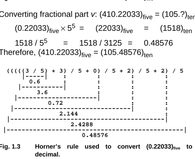
Converting fractional part v: (410.22033)_five = (105.?)_ten (0.22033)_five× 5⁵ = (22033)_five = (1518)_ten 1518 / 5⁵ = 1518 / 3125 = 0.48576

Therefore, (410.22033)_five = (105.48576)_ten

(((((3 / 5) + 3) / 5 + 0) / 5 + 2) / 5 + 2) / 5 |---| : : : : 0.6 : : : : |---| : : : 3.6 : : : |---| : : 0.72 : : |---| : 2.144 : |---|

2.4288

|---|

0.48576

Fig. 1.3 Horner’s rule used to convert (0.22033)_five to decimal.

(17)

1.6 Classes of Number Representations Integers (fixed-point), unsigned: Chapter 1 Integers (fixed-point), signed

signed-magnitude, biased, complement: Chapter 2 signed-digit: Chapter 3

(but the key point of Chapter 3 is

use of redundancy for faster arithmetic, not how to represent signed values) residue number system: Chapter 4

(again, the key to Chapter 4 is

use of parallelism for faster arithmetic, not how to represent signed values) Real numbers, floating-point: Chapter 17

covered in Part V, just before real-number arithmetic Real numbers, exact: Chapter 20

continued-fraction, slash, ... (for error-free arithmetic)

(18)

Part V Real Arithmetic

Part Goals

Review floating-point representations Learn about floating-point arithmetic Discuss error sources and error bounds Part Synopsis

Combining wide range and high precision Floating-point formats and operations The ANSI/IEEE standard

Errors: causes and consequences

When can we trust computation results?

Part Contents

Chapter 17 Floating-Point Representations Chapter 18 Floating-Point Operations

Chapter 19 Errors and Error Control

Chapter 20 Precise and Certifiable Arithmetic

(19)

17 Floating-Point Representations

Study representation method offering both wide range (e.g., astronomical distances) and high precision (e.g., atomic distances) Chapter Highlights

Floating-point formats and tradeoffs Why a floating-point standard?

Finiteness of precision and range The two extreme special cases:

fixed-point and logarithmic numbers Chapter Contents

17.1 Floating-Point Numbers

17.2 The ANSI/IEEE Floating-Point Standard 17.3 Basic Floating-Point Algorithms

17.4 Conversions and Exceptions 17.5 Rounding Schemes

17.6 Logarithmic Number Systems

(20)

17.1 Floating-Point Numbers

No finite number system can represent all real numbers Various systems can be used for a subset of real numbers Fixed-point ± w . f low precision and/or range Rational ± p / q difficult arithmetic

Floating-point ± s × b^e most common scheme

Logarithmic ± log_bx limiting case of floating-point Fixed-point numbers

x = (0000 0000 . 0000 1001)_two Small number y = (1001 0000 . 0000 0000)_two Large number Floating-point numbers

x = ± s × b^e or ± significand × base^exponent Two signs are involved in a floating-point number.

1. The significand or number sign,

usually represented by a separate sign bit 2. The exponent sign,

usually embedded in the biased exponent (when the bias is a power of 2,

the exponent sign is the complement of its MSB)

(21)

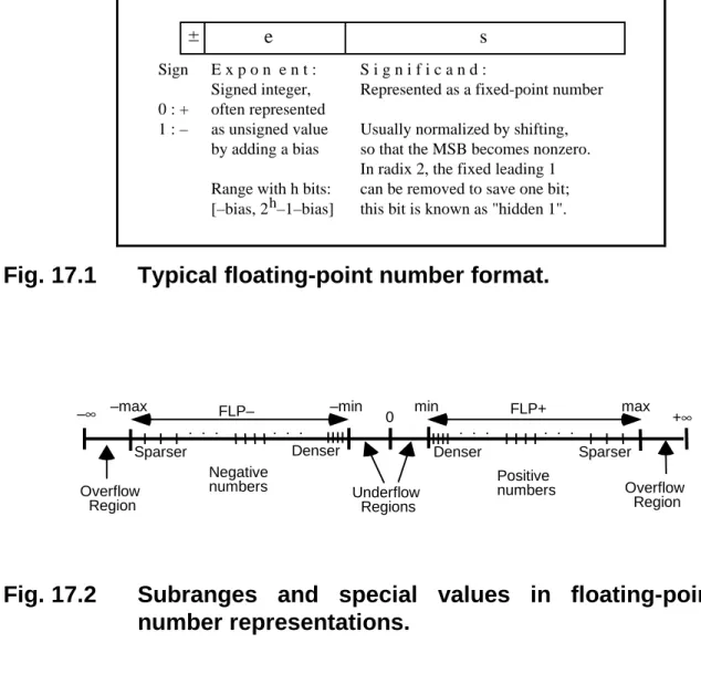
E x p o n e n t : Signed integer, often represented as unsigned value by adding a bias Range with h bits:

[–bias, 2 –1–bias]^h

S i g n i f i c a n d :

Represented as a fixed-point number Usually normalized by shifting, so that the MSB becomes nonzero.

In radix 2, the fixed leading 1 can be removed to save one bit;

this bit is known as "hidden 1".

Sign 0 : + 1 : –

± e s

Fig. 17.1 Typical floating-point number format.

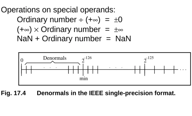
–∞ FLP– 0 FLP+ +∞

Underflow Regions Overflow

Region

Overflow Region max min

Denser Sparser

Positive numbers Negative

numbers

–max –min

Denser Sparser

. . . . . . . . . . . .

Fig. 17.2 Subranges and special values in floating-point number representations.

(22)

17.2 The ANSI/IEEE Floating-Point Standard

Short (32-bit) format

Long (64-bit) format

Sign Exponent Significand 8 bits,

bias = 127, –126to127

11 bits, bias = 1023,

–1022to1023

52 bits for fractional part (plus hidden 1 in integer part) 23 bits for fractional part

(plus hidden 1 in integer part)

Fig. 17.3 The ANSI/IEEE standard floating-point number representation formats.

(23)

Table 17.1 Some features of the ANSI/IEEE standard floating- point number representation formats

–––––––––––––––––––––––––––––––––––––––––––––––––

Feature Single/Short Double/Long

–––––––––––––––––––––––––––––––––––––––––––––––––

Word width (bits) 32 64

Significand bits 23 + 1 hidden 52 + 1 hidden Significand range [1, 2 – 2^–23] [1, 2 – 2^–52] Exponent bits 8 11

Exponent bias 127 1023

Zero (±0) e + bias = 0, f = 0 e + bias = 0, f = 0 Denormal e + bias = 0, f ≠ 0 e + bias = 0, f ≠ 0 represents ±0.f×2^–126 represents ±0.f×2^–1022 Infinity (±∞) e + bias = 255, f = 0 e + bias = 2047, f = 0 Not-a-number (NaN) e + bias = 255, f ≠ 0 e + bias = 2047, f ≠ 0 Ordinary number e + bias ∈ [1, 254] e + bias ∈ [1, 2046]

e ∈ [–126, 127] e ∈ [–1022, 1023]

represents 1.f × 2^e represents 1.f × 2^e min 2^–126 ≅ 1.2 × 10^–38 2^–1022 ≅ 2.2 × 10^–308 max ≅ 2¹²⁸ ≅ 3.4 × 10³⁸ ≅ 2¹⁰²⁴ ≅ 1.8 × 10³⁰⁸ –––––––––––––––––––––––––––––––––––––––––––––––––

(24)

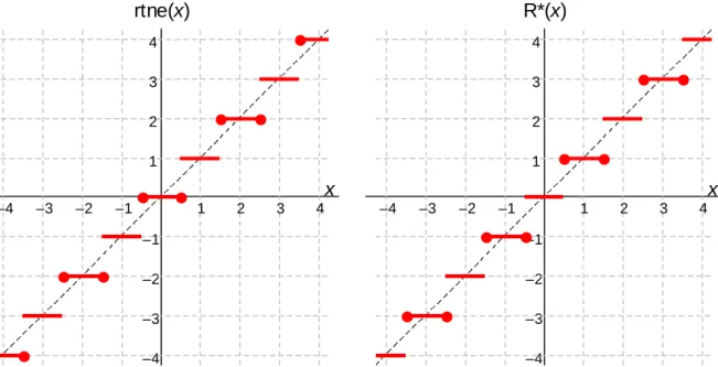
Operations on special operands:

Ordinary number ÷ (+∞) = ±0 (+∞) × Ordinary number = ±∞

NaN + Ordinary number = NaN

0 Denormals 2^–126

2^–125

. . . . . .

min

. . .

Fig. 17.4 Denormals in the IEEE single-precision format.

The IEEE floating-point standard also defines

The four basic arithmetic op’s (+, –, ×, ÷) and x must match the results that would be obtained if intermediate computations were infinitely precise Extended formats for greater internal precision

Single-extended: ≥ 11 bits for exponent ≥ 32 bits for significand bias unspecified, but exp range ⊇ [–1022, 1023]

Double-extended: ≥ 15 bits for exponent ≥ 64 bits for significand

exp range ⊇ [–16 382, 16 383]

(25)

17.3 Basic Floating-Point Algorithms Addition/Subtraction

Assume e1 ≥ e2; need alignment shift (preshift) if e1 > e2:

(±s1×bê1)+(±s2×bê2)=(±s1×bê1)+(±s2/bê1–e2)×bê1 = (±s1±s2/bê1–e1)×bê1= ±s×bê Like signs: 1-digit normalizing right shift may be needed Different signs: shifting by many positions may be needed Overflow/underflow during addition or normalization

Multiplication

(±s1×bê1) × (±s2×bê2) = ± (s1 × s2) × bê1+e2

Postshifting for normalization, exponent adjustment

Overflow/underflow during multiplication or normalization Division

(±s1×bê1) / (±s2×bê2) = ± (s1/s2) × bê1–e2 Square-rooting

First make the exponent even, if necessary √(s ×b^e) = s × b^e/2

In all algorithms, rounding complications are ignored here

(26)

17.4 Conversions and Exceptions Conversions from fixed- to floating-point Conversions between floating-point formats

Conversion from high to lower precision: Rounding ANSI/IEEE standard includes four rounding modes:

Round to nearest even [default rounding mode]

Round toward zero (inward) Round toward +∞ (upward) Round toward –∞ (downward) Exceptions

divide by zero overflow

underflow

inexact result: rounded value not same as original invalid operation: examples include

addition (+∞) + (–∞) multiplication 0 × ∞

division 0 / 0 or ∞ / ∞ square-root operand < 0

(27)

17.5 Rounding Schemes

Round

x_k–1x_k–2. . . x₁x₀. x_–1x_–2. . . x_–l

⇒

^yk–1y_k–2. . . y₁y₀. Special case: truncation or chopping

Chop

x_k–1x_k–2. . . x₁x₀. x_–1x_–2. . . x_–l

⇒

^xk–1x_k–2. . . x₁x₀.

chop(x)

–4 –3 –2 –1

x

–4 –3 –2 –1 1 2 3 4

4 3 2 1

chop(x)

–4 –3 –2 –1

x

–4 –3 –2 –1 1 2 3 4

4 3 2 1

Fig. 17.5 Truncation or chopping of a signed-magnitude number (same as round toward 0).

Fig. 17.6 Truncation or chopping of a 2’s-complement number (same as downward-directed rounding).

(28)

–4 –3 –2 –1

x

–4 –3 –2 –1 1 2 3 4

4 3 2 1

Fig. 17.7 Rounding of a signed-magnitude value to the nearest number.

Ordinary rounding has a slight upward bias

Assume that (x_k–1x_k–2. . . x₁x₀. x_–1x_–2)_two is to be rounded to an integer (y_k–1y_k–2. . . y₁y₀.)_two

The four possible cases, and their representation errors:

x_–1x_–2 = 00 round down error = 0 x_–1x_–2 = 01 round down error = –0.25 x_–1x_–2 = 10 round up error = 0.5 x_–1x_–2 = 11 round up error = 0.25

Assume 4 cases are equiprobable ⇒ mean error = 0.125 For certain calculations, the probability of getting a midpoint value can be much higher than 2^–l

(29)

rtne(x)

–4 –3 –2 –1

x

–4 –3 –2 –1 1 2 3 4

4 3 2 1

R*(x)

–4 –3 –2 –1

x

–4 –3 –2 –1 1 2 3 4

4 3 2 1

Fig. 17.8 Rounding to the nearest even number.

Fig. 17.9 R* rounding or rounding to the nearest odd number.

jam(x)

–4 –3 –2 –1

x

–4 –3 –2 –1 1 2 3 4

4 3 2 1

Fig. 17.10 Jamming or von Neumann rounding.

(30)

32×4-ROM-Round

x_k–1. . . x₄x₃x₂x₁x₀. x_–1. . . x_–l

⇒

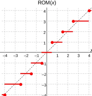
^xk–1 . . . x₄y₃y₂y₁y₀ . |–––––––––––| |––––––| ROM Address ROM Data

The rounding result is the same as that of the round to nearest scheme in 15 of the 16 possible cases, but a larger error is introduced when x₃ = x₂ = x₁ = x₀ = 1

ROM(x)

–4 –3 –2 –1

x

–4 –3 –2 –1 1 2 3 4

4 3 2 1

Fig. 17.11 ROM rounding with an 8 ×× 2 table.

(31)

We may need result errors to be in a known direction Example: in computing upper bounds,

larger results are acceptable,

but results that are smaller than correct values could invalidate the upper bound

This leads to the definition of directed rounding modes upward-directed rounding (round toward +∞) and downward-directed rounding (round toward –∞)

(required features of the IEEE floating-point standard)

up(x)

–4 –3 –2 –1

x

–4 –3 –2 –1 1 2 3 4

4 3 2 1

chop(x) = down(x)

–4 –3 –2 –1

x

–4 –3 –2 –1 1 2 3 4

4 3 2 1

Fig. 17.12 Upward-directed rounding or rounding toward +∞∞ (see Fig. 17.6 for downward-directed rounding, or rounding toward –∞∞).

Fig. 17.6 Truncation or chopping of a 2’s-complement number (same as downward-directed rounding).

(32)

17.6 Logarithmic Number Systems sign-and-logarithm number system:

limiting case of floating-point representation x = ±b^e × 1 e = log_b |x|

b usually called the logarithm base, not exponent base

Sign

Implied radix point e

±

Fixed-point exponent

Fig. 17.13 Logarithmic number representation with sign and fixed-point exponent.

The log is often represented as a 2’s-complement number (Sx, Lx) = (sign(x ), log₂|x|)

Simple multiply and divide; harder add and subtract Example: 12-bit, base-2, logarithmic number system 1 1 0 1 1 0 0 0 1 0 1 1

∆

Sign Radix point

The above represents –2^–9.828125 ≅ –(0.0011)_ten number range ≅ [–2¹⁶, 2¹⁶], with min = 2^–16

(33)

19 Errors and Error Control

Learn about sources of computation errors consequences of inexact arithmetic

and methods for avoiding or limiting errors Chapter Highlights

Representation and computation errors Absolute versus relative error

Worst-case versus average error Why 3 × (1/3) is not necessarily 1?

Error analysis and bounding Chapter Contents

19.1 Sources of Computational Errors 19.2 Invalidated Laws of Algebra

19.3 Worst-Case Error Accumulation

19.4 Error Distribution and Expected Errors 19.5 Forward Error Analysis

19.6 Backward Error Analysis

(34)

19.1 Sources of Computational Errors

FLP approximates exact computation with real numbers Two sources of errors to understand and counteract:

Representation errors

e.g., no machine representation for 1/3, 2 , or π Arithmetic errors

e.g., (1 + 2^–12)² = 1 + 2^–11 + 2^–24 not representable in IEEE format

We saw early in the course that errors due to finite precision can lead to disasters in life-critical applications Example 19.1: Compute 1/99 – 1/100

(decimal floating-point format, 4-digit significand in [1, 10), single-digit signed exponent)

precise result=1/9900≅1.010×10^–4(error≅10^–8or0.01%) x = 1/99 ≅ 1.010 × 10^–2 Error ≅ 10^–6 or 0.01%

y = 1/100 = 1.000 × 10^–2 Error = 0

z = x –_fp y = 1.010 × 10^–2 – 1.000 × 10^–2= 1.000 × 10^–4 Error ≅ 10^–6 or 1%

(35)

Notation for floating-point system FLP(r, p, A)

Radix r (assume to be the same as the exponent base b) Precision p in terms of radix-r digits

Approximation scheme A ∈ {chop, round, rtne, chop(g), ...}

Let x = r^es be an unsigned real number, normalized such that 1/r ≤ s < 1, and x_fp be its representation in FLP(r, p, A) x_fp = r^es_fp = (1 + η)x

A = chop –ulp < s_fp – s ≤ 0 –r × ulp < η ≤ 0 A = round –ulp/2 < s_fp – s ≤ ulp/2 |η| ≤ r × ulp/2

Arithmetic in FLP(r, p, A)

Obtain an infinite-precision result, then chop, round, . . . Real machines approximate this process by keeping g > 0 guard digits, thus doing arithmetic in FLP(r, p, chop(g))

(36)

Error analysis for FLP(r, p, A)

Consider multiplication, division, addition, and subtraction for positive operands x_fp and y_fp in FLP(r, p, A)

Due to representation errors, x_fp = (1 + σ)x , y_fp = (1 + τ)y x_fp ×_fp y_fp = (1 + η)x_fpy_fp = (1 + η)(1 + σ)(1 + τ)xy

= (1 + η + σ + τ + ησ + ητ + στ + ηστ)xy

≅ (1 + η + σ + τ)xy

x_fp /_fp y_fp = (1 + η)x_fp/y_fp = (1 + η)(1 + σ)x/[(1 + τ)y]

= (1 + η)(1 + σ)(1 – τ)(1 + τ²)(1 + τ⁴)( . . . )x/y

≅ (1 + η + σ – τ)x/y

x_fp +_fp y_fp = (1 + η)(x_fp + y_fp) = (1 + η)(x + σx + y + τy) = (1 + η)(1 + σ^{x +}τ^y

x + y )(x + y)

Since |σx + τy| ≤ max(|σ|, |τ|)(x + y), the magnitude of the worst-case relative error in the computed sum is roughly bounded by |η| + max(|σ|, |τ|)

x_fp –_fp y_fp = (1 + η^)(x_fp^{– y}_fp) = (1 + η)(x + σx – y – τy) = (1 + η)(1 + σ^{x –}τ^y

x – y )(x – y)

The term (σx – τy)/(x – y) can be very large if x and y are both large but x – y is relatively small

This is known as cancellation or loss of significance

(37)

Fixing the problem

The part of the problem that is due to η being large can be fixed by using guard digits

Theorem 19.1: In floating-point system FLP(r, p, chop(g)) with g ≥ 1 and –x < y < 0 < x, we have:

x +_fp y = (1 + η)(x + y) with –r^{–p +1} < η < r^–p–g+2 Corollary: In FLP(r, p, chop(1))

x +_fp y = (1 + η)(x + y) with |η| < r^–p+1

So, a single guard digit is sufficient to make the relative arithmetic error in floating-point addition/subtraction comparable to the representation error with truncation

(38)

Example 19.2: Decimal floating-point system (r = 10) with p = 6 and no guard digit

x = 0.100 000 000 × 10³y = –0.999 999 456 × 10² x_fp = .100 000 × 10³ y_fp = – .999 999 × 10² x + y = 0.544×10^–4 and x_fp + y_fp = 10^–4, but:

x_fp +_fp y_fp = .100 000 × 10³ –_fp .099 999 × 10³ = .100 000 × 10^–2

Relative error = (10^–3 – 0.544×10^–4)/(0.544×10^–4) ≅ 17.38 (i.e., the result is 1738% larger than the correct sum!) With 1 guard digit, we get:

x_fp +_fp y_fp = 0.100 000 0 × 10³ –_fp 0.099 999 9 × 10³ = 0.100 000 × 10^–3

Relative error = 80.5% relative to the exact sum x + y but the error is 0% with respect to x_fp + y_fp

(39)

19.2 Invalidated Laws of Algebra

Many laws of algebra do not hold for floating-point arithmetic (some don’t even hold approximately)

This can be a source of confusion and incompatibility Associative law of addition: a + (b + c) = (a + b) + c a = 0.123 41×10⁵ b = –0.123 40×10⁵ c = 0.143 21×10¹ a +_fp (b +_fp c)

= 0.123 41×10⁵ +_fp (–0.123 40×10⁵ +_fp 0.143 21×10¹) = 0.123 41 × 10⁵ –_fp 0.123 39 × 10⁵

= 0.200 00 × 10¹ (a +_fp b) +_fp c

= (0.123 41×10⁵ –_fp 0.123 40×10⁵) +_fp 0.143 21×10¹ = 0.100 00 × 10¹ +_fp 0.143 21 × 10¹

= 0.243 21 × 10¹

The two results differ by about 20%!

(40)

A possible remedy: unnormalized arithmetic a +_fp (b +_fp c)

= 0.123 41×10⁵ +_fp (–0.123 40×10⁵ +_fp 0.143 21×10¹) = 0.123 41 × 10⁵ –_fp 0.123 39 × 10⁵ = 0.000 02 × 10⁵ (a +_fp b) +_fp c

= (0.123 41×10⁵ –_fp 0.123 40×10⁵) +_fp 0.143 21×10¹ = 0.000 01 × 10⁵ +_fp 0.143 21 × 10¹ = 0.000 02 × 10⁵ Not only are the two results the same but they carry with them a kind of warning about the extent of potential error Let’s see if using 2 guard digits helps:

a +_fp (b +_fp c)

= 0.123 41×10⁵ +_fp (–0.123 40×10⁵ +_fp 0.143 21×10¹) = 0.12341×10⁵ –_fp 0.1233857×10⁵ = 0.24300×10¹ (a +_fp b) +_fp c

= (0.123 41×10⁵ –_fp 0.123 40×10⁵) +_fp 0.143 21×10¹ = 0.100 00 × 10¹ +_fp 0.143 21 × 10¹ = 0.243 21×10¹ The difference is now about 0.1%; still too high

Using more guard digits will improve the situation but does not change the fact that laws of algebra cannot be assumed to hold in floating-point arithmetic

(41)

Examples of other laws of algebra that do not hold:

Associative law of multiplication

a × (b × c) = (a × b) × c Cancellation law (for a > 0)

a×b = a×c implies b=c Distributive law a×(b+c) = (a×b)+(a×c) Multiplication canceling division

a × (b / a) = b

Before the ANSI-IEEE floating-point standard became available and widely adopted, these problems were exacerbated by the use of many incompatible formats

Example 19.3: The formula x = –b ± d, with d = b²– c , yielding the roots of the quadratic equation x²+2bx +c =0, can be rewritten as x = –c / (b ± d)

Example 19.4: The area of a triangle with sides a, b, and c (assume a ≥ b ≥ c) is given by the formula

A= s(s–a)(s–b)(s–c)

where s = (a+ b +c)/2. When the triangle is very flat, such that a ≅ b + c, Kahan’s version returns accurate results:

A = ¹₄ (a+(b+c))(c–(a–b))(c + (a–b))(a+(b–c))

(42)

19.3 Worst-Case Error Accumulation

In a sequence of operations, round-off errors might add up The larger the number of cascaded computation steps (that depend on results from previous steps), the greater the chance for, and the magnitude of, accumulated errors With rounding, errors of opposite signs tend to cancel each other out in the long run, but one cannot count on such cancellations

Example: inner-product calculation z =

∑

¹⁰²³_i=0 ^x⁽ⁱ⁾^y⁽ⁱ⁾

Max error per multiply-add step = ulp/2+ulp/2=ulp Total worst-case absolute error = 1024ulp

(equivalent to losing 10 bits of precision)

A possible cure: keep the double-width products in their entirety and add them to compute a double-width result which is rounded to single-width at the very last step

Multiplications do not introduce any round-off error Max error per addition = ulp²/2

Total worst-case error = 1024 × ulp²/2

Therefore, provided that overflow is not a problem, a highly accurate result is obtained

(43)

Moral of the preceding examples:

Perform intermediate computations with a higher precision than what is required in the final result

Implement multiply-accumulate in hardware (DSP chips) Reduce the number of cascaded arithmetic operations;

So, using computationally more efficient algorithms has the double benefit of reducing the execution time as well as accumulated errors

Kahan’s summation algorithm or formula

To compute s =

∑

^n–1_i=0 ^x⁽ⁱ⁾, proceed as follows s ← x⁽⁰⁾

c ← 0 {c is a correction term}

for i = 1 to n – 1 do

y ← x⁽ⁱ⁾ – c {subtract correction term}

z ← s + y

c ← (z – s) – y {find next correction term}

s ← z endfor

(44)

19.4 Error Distribution and Expected Errors MRRE = maximum relative representation error MRRE(FLP(r, p, chop)) = r^–p+1

MRRE(FLP(r, p, round)) = r^–p+1/2

From a practical standpoint, however, the distribution of errors and their expected values may be more important Limiting ourselves to positive significands, we define:

ARRE(FLP(r, p, A)) =

⌡

⌠

1/r 1

|x_fp – x|

x

dx x ln r 1/(x ln r) is a probability density function

0 1 2 3

1/2 3/4 1

Significand x 1 / (x ln 2)

Fig. 19.1 Probability density function for the distribution of normalized significands in FLP(r = 2, p, A).

(45)

19.5 Forward Error Analysis

Consider the computation y = ax + b and its floating-point version:

y_fp = (a_fp ×_fp x_fp) +_fp b_fp = (1 + η)y

Can we establish any useful bound on the magnitude of the relative error η, given the relative errors in the input operands a_fp, b_fp, and x_fp?

The answer is “no”

Forward error analysis =

Finding out how far y_fp can be from ax + b, or at least from a_fpx_fp + b_fp, in the worst case

(46)

a. Automatic error analysis

Run selected test cases with higher precision and observe the differences between the new, more precise, results and the original ones b. Significance arithmetic

Roughly speaking, same as unnormalized arithmetic, although there are some fine distinctions

The result of the unnormalized decimal addition .1234 × 10⁵ +_fp .0000 × 10¹⁰ = .0000 × 10¹⁰

warns us that precision has been lost c. Noisy-mode computation

Random digits, rather than 0s, are inserted during normalizing left shifts

If several runs of the computation in noisy mode yield comparable results, then we are probably safe d. Interval arithmetic

An interval [x_lo, x_hi] represents x, x_lo ≤ x ≤ x_hi

With x_lo, x_hi, y_lo, y_hi > 0, to find z = x / y, we compute [z_lo, z_hi] = [x_lo /_∇_fpy_hi, x_hi /_∆_fpy_lo]

Intervals tend to widen after many computation steps

(47)

19.6 Backward Error Analysis

Backward error analysis replaces the original question How much does y_fp deviate from the correct result y?

with another question:

What input changes produce the same deviation?

In other words, if the exact identity y_fp = a_altx_alt + b_alt

holds for alternate parameter values a_alt, b_alt, and x_alt, we ask how far a_alt, b_alt, x_alt can be from a_fp, b_fp, x_fp

Thus, computation errors are converted or compared to additional input errors

(48)

Example of backward error analysis y_fp = a_fp ×_fp x_fp +_fp b_fp

= (1 + µ)[a_fp ×_fp x_fp + b_fp] with |µ| <r^–p+1=r × ulp = (1 + µ)[(1 + ν)a_fpx_fp + b_fp] with |ν|<r^–p+1=r × ulp = (1 + µ)a_fp (1 + ν)x_fp + (1 + µ)b_fp

= (1 + µ)(1 + σ)a (1 + ν)(1 + δ)x + (1 + µ)(1 + γ)b

≅ (1 + σ + µ)a (1 + δ + ν)x + (1 + γ + µ)b

So the approximate solution of the original problem is the exact solution of a problem close to the original one

We are, thus, assured that the effect of arithmetic errors on the result y_fp is no more severe than that of r × ulp additional error in each of the inputs a, b, and x