A Quantitative information flow model for attribute-inference attacks and utility in data releases by sampling

A quantitative information flow model for attribute inference attacks and utility in sampling data publications. G643q Quantitative information flow model for attribute inference attacks and utility in sampling data releases [manuscrito] / Ramon Gonçalves Gonze — 2023.

Introduction

Contributions

We consider 3 adversaries with different prior knowledge (i.e., what is known before an attack is made) about the presence of the target in the sample release:. i). The model describes a data analyst trying to infer the distribution of attribute values ​​in the population.

Thesis outline

We provide closed formulas for prior and posterior vulnerabilities in attribute inference attacks and for prior utility loss. Although we do not present a closed formula for posterior utility loss of adversaries in Gf and for prior and posterior utility loss of adversaries in Gd, we provide an equation that can be computed in at most O(n3) and also an analysis of the behavior of these losses as as the sample or population size increases.

Background

Review on data disclosure control

The information "Bob is in the data set" does not itself cause damage to Bob if someone learns about him. Second, she asks how many people in the data set with a name other than T satisfyP, which returns y.

Quantitative Information Flow

• Secrets
• g-vulnerability
• Channels
• g-leakage

We have already seen that the opponent has a prior knowledge of the secret – a probability distributionπ∈DX. The posterior distribution δy∈DX (i.e. P r[X | Y=y]) represents the opponent's posterior knowledge of the set of secrets when she observes the output y.

General scenario

As discussed in Section 2.1, there are several indications in the literature that publishing data with very high levels of both privacy and usability is not feasible. After setting out the general scenario studied in this thesis, in the next section we begin to reason about the adversary's assumptions about population and then formalize the models based on the QIF framework that underpin our analyzes on privacy and utility in Chapter 4.

Assumptions about adversaries’ prior knowledge

The lack of knowledge in this situation is represented by a uniform distribution over all possible population datasets2. In this case, a dataset would be a set of independent and identically distributed random variablesX. a) Group of opponents Gf that assumes a uniform distribution over all possible frequencies of value in the population.

Adversary model for privacy analysis

• Group of adversaries G f
• Group of adversaries G d
• Adversary’s actions and system channel

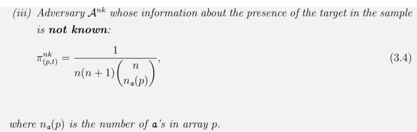
Privacy Analysis Adversary Model 35 where pis is the population array and t is the index of the target in p. We then define the previous distributions πin, πout, πnk for three different opponents with clear information about the presence of the target in the sample:. Adversary model for privacy analytics 37 (iii) AdversaryAnk whose information about the presence of the target in the sample.

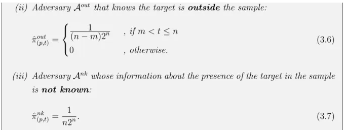
Finally, opponent Ank does not know anything about the target's presence in the sample, then the target's index can be both 1 or 2. The information that the target is in the sample for opponentAin, that the target is outside the sample for opponentWithout information about the target's presence in the sample for opponent Ank . We then define the prior distributionsπˆin,πˆout,πˆnk for three different adversaries with distinct information about the target's presence in the sample:.

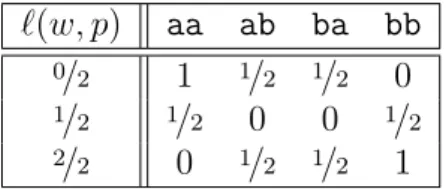
The adversary wants to infer the value of the target's attribute, so the set of possible guesses is W={a,b}. The expected probability that the adversary correctly guesses the value of the target's attribute after she observed the sample histogram”.

Adversary model for utility analysis

• Group of adversaries G f
• Group of adversaries G d
• Adversary’s actions and system channel

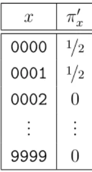
In the next two sections, we formally define adversary prior knowledge for two sets of adversaries that make different assumptions about the population data set (Section 3.2). Given the Xut secret set, the prior knowledge of the adversary, representing a data analyst trying to infer the frequency of the value a in the population, is the prior distribution of πut, defined as . In the next section, we precisely define the adversary's guesses about the distribution of attribute values ​​in the population and propose a loss function to measure the adversary's success.

We define Aut's success by looking at her uncertainty about the proportion of a's in the population. So if the opponent guesses what the exact true frequency in the population is, the loss will be 0. The opponent Aut can guess that there are 0, 1 or 2 people in the population with value a.

The input Sutp,y can be thought of as the probability that the histogram y will be published when the population is p, i.e. P r[y|p]. In this chapter, we present contributions related to ex-ante and ex-post vulnerabilities and utility losses for the models described in the last chapter.

Attribute inference attack

• Results on prior vulnerability
• Results on posterior vulnerability

Given the prior distributions πin, πout, and πnk on the set of secrets X, and the gain function g for attribute inference attack, the prior vulnerability, that is, the expected probability of adversaries Ain, Aout, and Ank, respectively, inferring the target's attribute value is Now we analyze the prior vulnerability to adversaries in Gd, whose prior knowledge is formalized by prior distributions ˆπin, ˆπout and ˆπnk. Now we show in Lemma4.1.5 that, when the prior distribution on secrets is πin, πout or πnk, the probability distribution on outputs (sampling histograms) is a uniform distribution.

Given the prior distributions of πin, πout, and πnk on the secret set X and the channel S, the probability that the sample histogram y∈ Y will be the result. Let X be the set of secrets, πin, πout, and πnk be the prior distributions on X, g be the gain function for the attribute inference attack, and S be the channel. Given the prior distributions of πin, πout, and πnk, the acquisition function g for the attribute inference attack, and the channel S, the posterior vulnerabilities are corresponding.

Given the set of secrets X, the prior distributions πˆin, ˆπout and ˆπnk and channel S, the marginal probability distribution on Y is Given the prior distribution πˆin, the gain function g for attribute inference attack and the channel S, the posterior vulnerability Vg[ˆπin ▷ S] which represents the expected probability that Ain correctly guesses the target's attribute value.

Data analyst and sample’s utility

• Results on prior utility loss
• Results on posterior utility loss

Using the lemmas above, we present a closed formula for prior utility loss Uℓ(πut) in Theorem 4.2.1. Recall that in the case of opponent Aut, this prior knowledge is defined by ˆπut. Given the past distribution πˆut on the set of secrets Xut and the loss function ℓ, the past vulnerability, i.e., is the expected probability that the data analyst's opponent infers the frequency of value a in the population.

Given the prior distribution of πut to the set of secrets Xut and the channel Sut, the probability that the histogram of the pattern y∈ Y will be the result is the same. Let πut be the prior distribution on the secret set Xut, g be the gain function for the attribute inference attack, and Sut be the channel. The Applicability of the Data and Sample Analyst 71 where δy,ut∈DXut is the intrinsic distribution when πut is the prior distribution and is the observed y (ie, P r[X|Y =y]).

Given the prior distribution πut, the loss function ℓ, and the channel Sut, the posterior vulnerability is Given the prior distribution πˆut in the set of secretsXut, the loss function ℓ, and the channel Sut, the posterior vulnerability, i.e., the expected probability that the data analyst's adversary infers the frequency of values ​​in the population after observing the histogram of sample is.

Discussion of results

On the right side of the y-axis we can also see by what factor the adversary is increasing her chance of correctly guessing the target's attribute after observing the sample. For example, m= 1 implies Vg[πin▷S] = 1 because there is only one person in the sample and the adversary knows that he is the target, so her chances of success will be doubled, i.e., L×g( πin, S) = 2. They confirmed a reasonable intuition that a person who was selected to be in the sample always has a higher probability of having his attribute value inferred by an adversary than a person who was not selected to be in the sample. was in the champion.

For adversaries Ain and Aout the impact is non-existent – ​​indeed Equations (4.18) and (4.19) in Theorem 4.1.3 depend only on the sample size m. We see that, as the sample size grows, the expected probability that Ank infers the trait value from its target also grows, and on the other hand, the data analyst's expected error decreases. Discussion of results 75 Figure 4.3: Vulnerabilities and utility losses for Ank andAutinGf forn= 500 and varying the sample size m.

Figure 4.4 shows the posterior vulnerabilities for adversaries inGd, and we see that the sampler is the one that suffers more damage to its privacy, that is, the adversary has a higher expected probability of correctly guessing its attribute value. Another interesting fact is that out-of-sample individuals have no harm to their privacy for adversaries in Gd, that is, Vg[ˆπout▷S] = Vg(ˆπout) = 1/2.

Conclusions

These vulnerabilities can be thought of as P r[X|Y =y] where X is the collection of secrets and Y is the collection of sample histograms. i) Opponent Ain and previous distribution πin: Vg(δin,y) = max. In the left summation, in the first elements of p there are ya's, and aspt=a, there will be y−1a's in the other m−1 positions, so we have m−1y−1. In the right summation, the reasoning is similar to the left one, except that nowpt =b, so there will be beyas in the other m−1 positions, so m−1y. ii) Opponent Aout and previous distribution πout: Vg(δout,y) = max.

In the first m elements of p there are y a's, so me. iii) Adversary Ank and prior distribution πnk: Vg(δnk,y) = max. We must count how many secrets (p, t)∈X satisfy the constraints pt=a∧na(p1..m)=y in the left summation within the maximum and pt=b ∧ na(p1..m)=y in the right summary within the max. m)=yin the left summation within the max and 1≤t≤m∧pt=b∧na(p1..m)=y in the right summation within the max.

In the right summation, the reasoning is similar to the left, except that nowpt =b, so there will beyas in the andrem−1 positions, so m−1y. ii) Resistor Aout and previous distribution πˆout: Vg(ˆδout,y) = max. m)=yin left summation within max andm

99 We have to count how many secrets (p, t)∈X satisfy the constraints pt=a∧na(p1..m)=y in the left summation within the max and pt=b ∧ na(p1..m)= y in the correct sum within the max.