Reserve in the Electricity Market

NOTICE: this is the author’s version of a work that was submitted for publication in Electric Power Systems Research. Changes resulting from the reviewing, publishing process, such as peer review, editing, corrections, structural formatting, and other quality control mechanisms may not be reflected in this document. Changes may have been made to this work since it was submitted for revision and publication. A definitive version was subsequently accepted and published in Electric Power Systems Research, DOI: 10.1016/j.epsr.2013.08.006

Optimization Models for an EV Aggregator Selling Secondary

1

Reserve in the Electricity Market

2 3

R.J. Bessa^* and M.A. Matos 4

INESC TEC - INESC Technology and Science (formerly INESC Porto) and FEUP - Faculty of Engineering, University of Porto, 5

Portugal 6

7

Abstract

8

Power system regulators and operators are creating conditions for encouraging the participation of the 9

demand-side into reserve markets. The electric vehicle (EV), when aggregated by a market agent, holds 10

sufficient flexibility for offering reserve bids. Nevertheless, due to the stochastic nature of the drivers’

11

behavior and market variables, forecasting and optimization algorithms are necessary for supporting an 12

EV aggregator participating in the electricity market. This paper describes a new day-ahead optimization 13

model between energy and secondary reserve bids and an operational management algorithm that 14

coordinates EV charging in order to minimize differences between contracted and realized values. The 15

use of forecasts for EV and market prices is included, as well as a market settlement scheme that includes 16

a penalty term for reserve shortage. The optimization framework is tested in a test case constructed with 17

synthetic time series for EV and market data from the Iberian market.

18 19

Keywords: Electric vehicle, aggregator, optimization, electricity market, secondary reserve, regulation 20

reserve.

21 22

Nomenclature

23

µ: ratio between upward and downward secondary reserve;

24

Ѱ: costs associated to deviations between actual charging and accepted bids;

25

φ: convex loss function;

26

Ф: costs associated to reserve shortage;

27

α: penalization coefficient for secondary reserve capacity shortage;

28

γ: penalization coefficient for reserve not supplied (electrical energy);

29

∆t: time step (length of the time interval) of time interval t;

30

E_t: optimized electrical energy for time interval t;

31

E_t,j: optimized electrical energy for charging the j^th EV in time interval t;

32

*Correspondence to: Ricardo Bessa, INESC Porto, Campus da FEUP, Rua Dr. Roberto Frias, 378, 4200 - 465 Porto Portugal. Telf:

+351 22 209 4208. Fax: +351 22 209 4050. E-mail: [email protected]

E^*_t,j: electrical energy consumed by the j^th EV in time interval t;

33

H: set of time intervals from the optimization horizon;

34

plug

Hˆj : forecasted availability (or plugged-in) period of the j^th EV;

35

plug

Hj : availability (or plugged-in) period of the j^th EV;

36

λtup: number of equivalent minutes of dispatched upward reserve in interval t;

37

λtdown: number of equivalent minutes of dispatched downward reserve in interval t;

38

M_t: total number of EV plugged-in at time interval t;

39

πt-: negative imbalance unit cost of time interval t;

40 πt

+: positive imbalance unit cost of time interval t;

41

P_j^max: maximum charging power of the j^th EV;

42

max t0

P : maximum, constant and feasible charging power of the EV fleet in time interval t₀. 43

min t0

P : minimum, constant and feasible charging power of the EV fleet in time interval t₀. 44

down j

Pt_, : downward secondary reserve power of the j^th EV for time interval t;

45

up j

Pt_, : upward secondary reserve power of the j^th EV for time interval t;

46

t0

P′: operating point (or actual preferred operating point);

47

down

Pt

0′ : available downward secondary reserve power;

48

up

Pt

0′ : available upward secondary reserve power;

49

down

Pt

0 : downward secondary reserve power that can be sustained during interval t;

50

up

Pt

0 : upward secondary reserve power that can be sustained during interval t;

51

upper

Pt

0 : upper power limit that guarantees full availability of downward reserve power in time interval t₀; 52

lower

Pt

0 : lower power limit that guarantees full availability of upward reserve power in time interval t₀; 53

p_t^surplus: price for positive imbalances of time interval t;

54

p_t^shortage: price for negative imbalances of time interval t;

55

pˆt: day-ahead energy price forecast for time interval t;

56

cap

pˆt : forecasted capacity price of secondary reserve;

57

down

pˆt : forecasted price for dispatched downward reserve;

58

up

pˆt : forecasted price for dispatched upward reserve;

59

p_t: day-ahead energy price for time interval t;

60

Rˆj: forecasted charging requirement of the j^th EV;

61

j

Rt_,

0 : residual charging requirement of the j^th EV at beginning of time instant t₀; 62

down

RNSt : downward reserve not supplied in time interval t;

63

up

RNSt : upward reserve not supplied in time interval t;

64

T: time interval of the last plugged-in EV to depart;

65

t_final: last time interval of the availability period;

66

t_initial: first time interval of the availability period;

67

v_k: slack variable;

68

1. Introduction

69

The participation of loads in ancillary services markets has gained relevance in the recent years [1], in 70

particular with the deployment of the smart-grid concept with bidirectional communication [2]. The 71

electric vehicle (EV), when aggregated by a market agent, is a suitable candidate for selling reserve 72

services in the electricity market [3].

73

Secondary (or regulation) reserve consists in loads and generators under direct real-time control of the 74

system operator (SO), via automatic generation control (AGC), for increasing or decreasing 75

generation/consumption. The response time is very fast (e.g., less than 30 seconds) and is used to bring 76

back the frequency and the interchange programs to their nominal values (i.e., reduce the area control 77

error – ACE).

78

The current market rules do not allow the participation of small loads and generators (e.g., the 79

minimum bid is generally around megawatts),and even if small bids are allowed, the AGC would need to 80

send control signals to each EV supplying secondary reserve.

81

The solution proposed by several authors is an EV aggregator acting as an intermediary between EV 82

drivers, the electricity market and the SO [4][5]. Almeida [6] describes a control scheme for integrating 83

aggregated EV in the AGC operation of interconnected systems. In this framework, the AGC sends set- 84

points to aggregators that, afterwards, distribute individual set-points among the plugged-in EV. This 85

reduces significantly the communication burden and increases its reliability.

86

The work of this paper explores a solution where the EV aggregator controls directly the charging of 87

EV plugged-in in slow charging points and sells secondary reserve power in the electricity market.

88

The vehicle-to-grid (V2G) mode was not considered in this paper. Instead, the reserve is supplied by 89

establishing a preferred operating point (POP) [7]. The POP consists in the EV consumption level that can 90

be increased (downward reserve) or decreased (upward reserve) limited by zero and by the maximum 91

charging power. For instance, an EV charging at 2kW could provide 2 kW of upward regulation until it 92

reaches “zero load” and 1 kW of downward regulation if the maximum charging power is 3 kW.

93

Compared to V2G, this solution does not require additional investment in equipment, and it reduces the 94

costs with battery wear and losses in the charger [7].

95

Different algorithms for supporting the participation of EV in the reserve market were proposed in the 96

literature. Sortomme and El-Sharkawi [8] propose three heuristic strategies and equivalent optimal 97

analogues to define the POP and regulation reserve bids of an EV aggregator. Han et al. [9] describe a 98

dynamic programming based algorithm to calculate regulation power bids from EV. Rotering and Ilic 99

[10] describe two dynamic programming optimization algorithms for an optimal controller installed in an 100

EV. One algorithm optimizes the charging rates and periods for minimizing the cost, and the other 101

maximizes the profit from selling regulation power. Wu et al. [11] discuss pricing schemes to induce the 102

participation of EV in frequency regulation services.

103

All the aforementioned algorithms assume that perfect forecasts are available for all the variables. In 104

fact, when designing bidding optimization models, it is necessary to consider the need to forecast these 105

variables and the occurrence of forecast errors. Pantos [12] presents a stochastic optimization algorithm 106

for the participation in the electricity market (energy and regulation reserve), which includes uncertainties 107

related to the market price and driver’s behavior. Han et al. [13] propose a probabilistic model for 108

modeling the achievable power capacity of an EV aggregator when providing regulation reserve. Bessa et 109

al. [14] described an optimization model for energy and secondary reserve bids. A naïve forecasting 110

approach was used for producing forecasts for aggregated values of the EV variables. Bessa and Matos 111

[15] compared two alternative approaches to optimize the participation of an EV aggregator in the day- 112

ahead energy market (reserve was not considered). The two algorithms use, as input, forecasts for the EV 113

variables produced by statistical models. The same authors present in [16] a day-ahead optimization 114

model and operational management algorithms for day-ahead and hour-ahead manual (or balancing) 115

reserve bids.

116

Compared to Pantos [12] and Han et al. [13], the optimization approach proposed in this present paper 117

characterizes the EV individually, which as shown in [15], provides a more accurate representation and 118

coordinates the EV individual charging for mitigating forecast errors. Furthermore, the formulation of the 119

optimization models proposed in this present paper contemplates the specific characteristics of secondary 120

reserve. For instance, the models that will be described in section 3 are formulated to be robust to the 121

variability (in size and direction) of the net electrical energy from the secondary reserve dispatch. The 122

influence of forecast errors is also studied, in particular its impact on reserve shortage situations, and a 123

market settlement scheme with a penalty term for reserve shortage situations is also proposed. Finally, an 124

operational management algorithm is also described, which is essential to coordinate the EV charging 125

during the operating hour to comply with the market commitments, while in [12] this was identified as 126

future work.

127

Compared to the approach described by Bessa et al. [14], the present paper makes several innovations:

128

the formulation of the optimization problem includes the possibility of offering a reserve band in both 129

upward and downward directions; it disregards the need to forecast the reserve direction and participation 130

factor; the optimization uses forecasts for each EV; an operational management algorithm is proposed for 131

coordinating EV charging and for minimizing the difference between contracted and realized values of 132

energy and reserve. Compared to the approach described by Bessa and Matos [16] for the manual reserve, 133

the day-ahead and operational management problems described in this paper are different, since they were 134

developed taking into account the characteristics of secondary reserve. For example, the proposed day- 135

ahead optimization model does not derive the reserve bids based on the forecasted reserve direction (that 136

was found to be almost random), but it offers a reserve band in both directions and the operational 137

management algorithm is based on a strategy that redefines the EV fleet’s operating point in order to 138

maximize the available secondary reserve.

139

The remaining of the paper is organized as follows: section 2 describes the problem and the specific 140

characteristics of secondary reserve; section 3 formulates the day-ahead optimization problem; section 4 141

describes the operational management algorithm and how the aggregator redefines the EV fleet’s 142

operating point; section 5 proposes two new market settlement schemes; the test case results are presented 143

and discussed in section 6; section 7 presents the overall conclusions.

144

2. Problem Description

145

2.1 Electricity Market Framework 146

The EV aggregator participates in the day-ahead electrical energy market with bids to purchase energy, 147

which are paid at a single marginal price.

148

In addition to this market session, a day-ahead session for secondary reserve capacity is also 149

considered. Two examples of market sessions for this reserve type are the secondary reserve market in the 150

Iberian electricity market (MIBEL) [17] and the regulation reserve market in CAISO (California ISO) 151

[18].

152

This reserve is generally contracted in a day-ahead basis (e.g. Portugal, Spain, Italy and the Alberta 153

region), and even in markets with hour-ahead sessions, a major fraction of the reserve is contracted day- 154

ahead (see the case of CAISO [18]). There are two possible market-clearing schemes: a sequential market 155

(typically European markets) where the energy market takes place first, followed by a market for 156

secondary reserve; a market where energy and reserve requirements are jointly cleared (typically U.S.

157

markets). The approach described in this paper makes no distinction between these two schemes, but a 158

sequential market-clearing is assumed in this paper since the Iberian market is used as test case in section 159

6.

160

The aggregator presents a bid with a reserve band (in MW) that is divided into upward and downward 161

directions, and the reserve is remunerated with two prices: available capacity price (in €/MW) that results 162

from the capacity allocation of the secondary reserve market; dispatched capacity price (in €/MWh) that 163

may result from the balancing market.

164

The aggregator is a price-taker, which means that the bids made by the aggregator do not affect the 165

market-clearing price of energy and reserve. The price-taker assumption is valid when there is sufficient 166

competition in the market and a single market agent does not have a large quota of the market (i.e., 167

market power). Nevertheless, if the size of the aggregator’s bid becomes significant, even if it remains a 168

price-taker, it will shift the merit order curve and change the market-clearing price. In this case, it is not 169

possible to decouple the price forecast from the buying/selling bids computed with the optimization 170

problem.

171

In general, the electricity markets have hourly or half-hourly time steps. For the secondary reserve 172

market, the power in the reserve bid is assumed to be constant during the market interval. An EV 173

aggregator may not be able to offer constant power during a complete hour because several EV can depart 174

and arrive during that interval. For instance, the aggregator can have 1000 EV plugged-in during a half- 175

hour and 800 EV during the second half-hour. If all EV are charging at 2 kW (but with a maximum 176

charging power of 3 kW), the aggregator can offer 1MW of downward reserve in the first half-hour and 177

0.8 MW in the second. However, in an hourly time interval, the average power would be 0.9 MW, which 178

can only be attained during the first half-hour.

179

Therefore, in this paper a change in the current market rules is assumed to promote the participation of 180

EV in secondary reserve. The market time interval remains one hour, which means that from the market- 181

clearing it results an hourly price, but the secondary reserve bid submitted by the EV aggregator is 182

decomposed in sub-hourly intervals of predefined length ∆t and with constant power. In the 183

aforementioned example, assuming ∆t equal to 30 minutes, the downward reserve bid would be: 1 MW 184

for the first half-hour and 0.8 MW for the second. The time length ∆t is a predefined value and it should 185

be defined in accordance to the average trip duration time. Note that most of the electricity markets 186

created complex bids to accommodate specific characteristics of conventional generation units (e.g., 187

minimum run times). Thus, this can be seen as an additional complex bid designed for EV aggregators 188

(and also for other types of flexible loads). This change demands a new market-clearing algorithm that 189

takes into account complex bids from the EV aggregator.

190

2.2 Characteristics of the Secondary Reserve 191

In the absence of perturbations, the events handled by secondary reserve are usually minute-to-minute 192

random fluctuations inside the operating period, but in some cases, this reserve can also be used to handle 193

large deviations between load and generation (e.g. unplanned outage or loss of synchronism from a 194

generator). Despite being contracted on an hourly basis, the secondary reserve is mobilized for short 195

periods-of-time (e.g., 5 minutes). Secondary reserve must only be used to correct the ACE and not for 196

other purposes, such as to minimize unintentional energy imbalances [19].

197

This contrasts with manual (or balancing) reserve that is frequently used for periods of more than one 198

hour to solve energy imbalances, such as forecast errors from renewable energy. According to Hirst [20], 199

manual reserve (called load-following by the author) differs from secondary (called regulation by the 200

author) in two important aspects: (a) it is used over long periods of time compared to secondary reserve;

201

(b) the changes in reserve direction are frequently predictable and have similar daily patterns [16].

202

This reserve has specific characteristics that must be considered when developing optimization models 203

for an EV aggregator.

204

The first characteristic is that, despite being contracted on an hourly basis, secondary reserve is 205

normally not dispatched in the same direction during the complete hour. In an hourly period, the reserve 206

can be dispatched in one direction during a period below one hour (e.g., upward reserve during 40 207

minutes), while in other cases, it can be dispatched in both directions (e.g., 10 minutes of upward and 50 208

minutes of downward reserve).

209

Figure 1 depicts the histograms for the number of equivalent minutes of dispatched secondary upward 210

reserve of a hydro and a thermal power plant in Portugal. The number of equivalent minutes corresponds 211

to the ratio between the dispatched reserve power (energy in MWh) and its available reserve power 212

(power in MW).

213

Figure 1: Histograms for the number of equivalent minutes of the upward secondary reserve of a hydro (Alqueva) and thermal (Lares) power plants in Portugal for the year 2011.

The two histograms show a wide variation of the number of equivalent minutes. This means that, when 214

making a reserve bid, the aggregator does not know, with certainty, the reserve dispatch duration. For 215

example, for a downward reserve bid of 1 MW, a value of 20 minutes in the histogram corresponds to 216

dispatching this reserve power only during 20 minutes and no dispatch in the remaining 40 minutes and, 217

in this case, the EV fleet only charges 0.33 MWh of electrical energy (instead of the expected 1 MWh). In 218

contrast to generation units, this creates a problem for EV since their charging requirements must be 219

satisfied and the aggregator does not know beforehand, with certainty, the quantity of electrical energy 220

charged as downward reserve. The same is valid for upward reserve.

221

The number of equivalent minutes of dispatched secondary reserve is generally low. For instance, the 222

annual average value of the hydropower plant is 22 minutes for upward and 24 minutes for downward 223

secondary reserve.

224

A second characteristic, and in contrast to the assumption made in literature about the EV aggregator 225

participation in the secondary reserve market (see for instance reference [9]), is that the net electrical 226

energy from reserve provision in each hour is different from zero. Figure 2a depicts the histogram of the 227

total net energy of secondary reserve in Portugal, during the year 2011. As shown in the histogram, the 228

net energy is frequently different from zero. An asymmetrical regulation signal adds uncertainty to the 229

battery state of charge after each hour.

230

Figure 2: (a) Histogram of the net electrical energy of secondary reserve in Portugal for the year 2011 (negative value is upward reserve, positive is downward reserve); (b) Autocorrelation function (ACF) of the

net electrical energy of secondary reserve in Portugal for the year 2011.

A third characteristic, and linked to the second one, is that it is challenging to produce forecasts with 231

acceptable accuracy for this net energy. Figure 2b depicts the autocorrelation plot of the total net energy 232

of secondary reserve in Portugal, during the year 2011. This plot shows an autocorrelation below 0.25 for 233

all time lags, and the value for t-1 is only around 0.25. This low value of serial dependency suggests that 234

there is a low amount of information in the past values of the time series, which makes it challenging to 235

produce forecasts with acceptable accuracy. This is consistent with the expected random nature of the 236

secondary reserve dispatch.

237

To conclude, the analyses conducted in this section showed the following:

238

• the duration period of the dispatched reserve is variable, and in general, lower than one hour;

239

• the net energy from the reserve dispatch is frequently different from zero, and it is difficult to 240

forecast its value with acceptable accuracy.

241

Therefore, the formulation of the day-ahead optimization problem, which will be presented in section 242

3, should include constraints that allow a degree of flexibility in handling situations where the available 243

reserve in the previous intervals was not dispatched in one direction (on the contrary to what was planned 244

by the aggregator) or was dispatched only for a limited period of time in one direction.

245

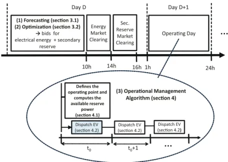
2.3 Participation in the Electricity Market 246

Figure 3 depicts the sequence of tasks for the participation in the day-ahead energy and secondary 247

reserve markets. The gate closure and period for submitting bids are the ones from the Iberian electricity 248

market.

249

Figure 3: Sequence of tasks for the participation in the day-ahead energy and secondary reserve markets.

In the first phase, the aggregator, at day D, forecasts the EV charging requirement and availability, the 250

energy, and reserve prices (described in section 3.1). This forecasted information is the input, in a second 251

phase, of a day-ahead optimization model (for next day D+1) that computes the bids for the energy and 252

secondary reserve markets (described in section 3.2).

253

During the operating day (day D+1), before the beginning of each time interval t0 (with length ∆t), the 254

aggregator redefines the EV fleet operating point, computes the available upward and downward reserve 255

power, and communicates this information to the SO (described in section 4.1). The aggregator dispatches 256

the EV for meeting the fleet’s operating point for each time interval (t₀, t₀₊₁,…) and places the plugged-in 257

EV on standby to supply upward and downward reserve in response to an AGC request. An operational 258

management algorithm is used to coordinate the EV charging (described in section 4.2). A penalty term is 259

applied for cases with reserve power shortage.

260

3. Day-ahead Energy and Reserve Optimization

261

Section 2.2 discussed the characteristics of secondary reserve and concluded that it is not possible to 262

produce forecasts with acceptable quality for the hourly AGC regulation signal. Thus, the formulation of 263

the day-ahead optimization problem described in this section disregards this information, and the goal is 264

to obtain robust solutions that assure an acceptable reliability of the secondary reserve provision as well 265

as an attractive income to the aggregator and the EV in its portfolio.

266

The algorithm uses, as input, forecasts for several variables that are briefly described in section 3.1.

267

3.1 Input Variables and Forecasts 268

The EV load is modeled with two variables: availability period and charging requirement. The EV 269

availability is the time-period when the EV is plugged-in for charging. It is a binary variable indicating 270

whether or not the EV is plugged-in for charging in each time interval with length ∆t.

271

The charging requirement of the EV is the total energy needed to get from the initial state-of-charge 272

(SOC) (i.e., when the EV arrives for charging) to the target SOC defined by the EV driver for the next 273

trip, including the losses from the charger. A charging requirement value is always associated to an 274

availability period. For example, an EV with battery size of 24 kWh parking with a 50% SOC (12 kWh) 275

and with target SOC of 100%, needs 12 kWh to reach full battery plus 1.33 kWh of charger losses. Thus, 276

the charging requirement is 13.33 kWh.

277

These variables are obtained from the advanced metering infrastructure installed in households. In this 278

framework, it is assumed that the EV driver, when plugged-in for charging, communicates the target SOC 279

and expected departure hour to the aggregator. If this information is not communicated, the aggregator 280

will assume a target SOC of 100% by default.

281

The availability period is a binary time series forecasted with a generalized linear model (GLM) [21]

282

with the response variable following a binomial distribution. After forecasting the availability period, the 283

corresponding charging requirement is forecasted with non-parametric bootstrapping. A complete 284

description of the forecasting algorithm can be found in [15].

285

The day-ahead energy price is forecasted with an additive model (using cubic splines) and using the 286

following variables as explanatory variables: lagged variables of the price (i.e., t-1, t-2, t-3), forecasted 287

wind power penetration, periodic function for the hour of the day and day of the week.

288

The secondary reserve has two prices: price for available reserve capacity and price for dispatched 289

reserve. The price for available reserve capacity is forecasted with an ARIMA model selected using the 290

function auto.arima R package forecast [22]. The price for dispatched reserve is an irregular time series 291

forecasted with the Holt-Winters model with trigonometric functions [23].

292

3.2 Formulation of the Optimization Model 293

The decision variables of the optimization problem are: optimized energy (E_t,j) for charging the j^th EV 294

in time interval t (i.e., the preferred operation point – POP), the upward and downward secondary reserve 295

power (P_t,j^down and P_t,j^up) of the j^th EV for time interval t. The energy and reserve bids are the sum of the 296

individual values of each EV (i.e., the decision variables associated to each EV - E_t,j, P_t,j^down and P_t,j^up).

297

The optimization problem is formulated assuming that there is a single reserve capacity price. In 298

markets with separated sessions for upward and downward secondary reserve, the modification would be 299

a different capacity price for each direction.

300

The objective function is the minimization of the total cost, and it has the following components: (a) 301

cost of purchasing energy; (b) income from reducing the consumption (dispatched upward reserve); (c) 302

cost from charging EV as downward reserve; (d) income from having available secondary reserve power.

303

It can be written as:

304

( ) ( )

( ) ( )

∑ ∑ ∑

∑ ∑

∈

=

=

= =

 







 







+

⋅

−

∆

⋅

⋅

+

∆

⋅

⋅

−

⋅

H

t M

j

down j t up

j t cap

t M

j

down j t down

t

M j

M j

up j t up

t j t t

t t

t t

P P p

t P

p

t P p

E p

1 , ,

1 ,

1 , 1 ,

ˆ ˆ

ˆ ˆ

min

305

where

pˆ is the forecasted energy price, t pˆ is the forecasted price for dispatched upward reserve, _t^up 306

down

pˆt is the forecasted price for dispatched downward reserve, ^cap

pˆt is the forecasted price for available 307

reserve capacity, M_t is the number of EV plugged-in at time interval t, ∆t is the length of time interval t, H 308

is the set of time intervals of the optimization period (e.g., for one day with ∆t=0.5 hr, H ranges between 1 309

and 48).

310

The constraints of the optimization problem are described in the following paragraphs.

311

The method for computing the reserve band is as follows: first, the charging requirements are satisfied 312

considering the purchased energy and the upward reserve band, and then, the downward capacity is the 313

remaining capacity (below the maximum charging power, P_t^max) in each time interval t.

314

The first point leads to the following constraint:

315

( )

{

}

H t

up j t j

t

P t R j M

E

plug j

, , 1 ˆ ,

ˆ ,

−

⋅ ∆ = ∀ ∈ ⋯

∑

316

where

i

Rˆ is the forecasted charging requirement of the jj_, ^th EV, and ^plug

Hˆj is the forecasted availability 317

period of the j^th EV.

318

The second point leads to the following constraint for downward reserve:

319

{ ^M } ^{t H}

j P P

t

E

∆ +

≤

, ∀ ∈ 1 , ⋯ ,

, ∀ ∈

320

The upward reserve band is limited by the energy bid in each time interval:

321

( ^{E t} ) ^{j { M } t H}

P

≤

∆ , ∀ ∈ 1 , ⋯ ,

, ∀ ∈

322

and its total is limited by the charging requirement in each availability period:

323

( )

{

}

H t

up j

t

t R j M

plug

P

j

, , 1 ˆ ,

ˆ ,

⋅ ∆ ≤ ∀ ∈ ⋯

∑

324

Constraint (5) is included to avoid the aggregator from offering a total upward reserve greater than the 325

total energy that the EV fleet can consume (i.e., the charging requirement). For example, without this 326

constraint, an EV parked for 10 hourly intervals with a forecasted charging requirement of 1.5 kWh could 327

offer upward reserve in 9 intervals. This would give

^∑

( )

( )

∑

Hj t

up j

t t kWh

ˆ P, 91.5 13.5 for meeting the charging requirement. If in one of these intervals 329

upward reserve is not dispatched, this strategy would harm significantly the reliability of upward reserve 330

and increase the penalty costs for reserve shortage (topic that will be discussed in section 5); the inclusion 331

of constraint (5) limits

∑

(

)

Hj t

up j

t t kWh

ˆ P, 1.5 .

332

The total downward reserve is also constrained by the charging requirement:

333

( )

{

}

H t

down j

t

t R j M

P

plug j

, , 1 ˆ ,

ˆ ,

⋅ ∆ ≤ ∀ ∈ ⋯

∑

334

With the constraint (7), the aggregator can only offer upward reserve in a specific interval if the EV is 335

able to offer an energy bid (E_k,j) with the corresponding quantity both in the same and subsequent time 336

intervals. This increases the robustness of the bidding optimization since it forces the EV to be capable of 337

consuming the quantity that is offered as upward reserve. Otherwise, considerable penalization (topic 338

discussed in section 5) could be incurred if upward reserve cannot be supplied. This constraint consists in 339

postponing EV charging by offering upward reserve:

340

( ^{P t} )

( ) ^E

^{j { M}

^{} t H}

k t k

up j k

final

final

⋅ ∆ ≤ ∑ ∀ ∈ ∀ ∈

∑

^{2 , 1 ,} ⋯ ^{, ,}

341

where t_final is the last time interval of the forecasted availability period, i.e. ^plug

j

final H

t ∈ ˆ . 342

In (7), the total consumption reduction between t and t_final must be below or equal to half of the energy 343

bid in the same period. For example, if the aggregator in time interval t=1 offers an energy and upward 344

reserve bid of 1.5 kW, it must present an additional energy bid of 1.5 kWh in any interval t>1 of the 345

availability period, otherwise the constraint is violated.

346

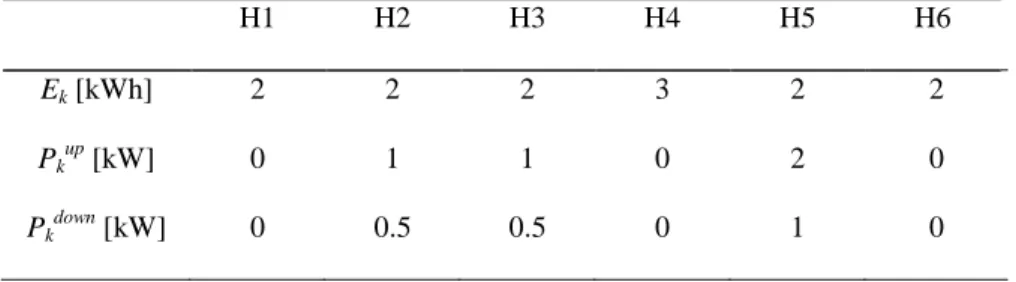
In order to illustrate this constraint, Table 1 presents two candidate solutions for offering upward 347

reserve with an EV plugged-in during six hours (i.e, ∆t=1 hour) and with a charging requirement of 9 348

kWh and maximum charging power of 3 kW.

349

Table 1: Set of charging solutions of an EV offering upward reserve power in a six-hour availability period with a charging requirement of 9 kWh.

Solution (a), with constraint (7), is unfeasible because the charging requirement is already satisfied 350

after interval H3, and the aggregator makes an upward reserve offer in intervals H5 and H6 where it is not 351

able to supply if requested by the TSO.

352

Solution (b) is feasible. For instance, in interval H3 the EV offers 3 kW of upward reserve, and it 353

consumes additional 3 kW in the remaining time intervals (H4 in this case).

354

It is important to stress that constraint (7) offers robust solutions since the available reserve power in 355

the current interval is not affected even if the upward reserve is dispatched in lower quantities during 356

previous intervals. For instance, if the reserve in interval H1 of solution (b) is not fully dispatched, there 357

would be a surplus of consumed electrical energy compared to what was planned, but the aggregator can 358

consume less in interval H2 (if necessary) to compensate this surplus at a cost of an energy imbalance 359

penalty.

360

The reserve band is divided into upward and downward directions with the following equality:

361

{ ^{1 , ,} } ^{, ,}

,

,

,

P j M t H

P

= µ ⋅

∀ ∈ ⋯

∀ ∈

362

In the Iberian market, the reserve band is divided into 2/3 for upward and 1/3 for downward, so the 363

value of µ is 2. In markets without a rule for splitting the reserve band, the value of µ can be defined by 364

considering the reserve prices, or the reserve reliability (e.g., estimate a µ from historical data that leads 365

to the minimum reserve shortage), or a trade-off between both criteria.

366

The optimization problem of Equations (1)-(8) is an LP problem that can be solved using any 367

commercial or non-commercial LP solvers.

368

After, solving the LP problem, a post-processing phase is applied to the downward reserve band. In 369

order to create sufficient flexibility for supplying upward reserve, the purchased energy is higher than the 370

charging requirement [see equation (2)]. Thus, a post-processing phase is necessary to eliminate 371

downward reserve bids from the time intervals where the total purchased energy is above the charging 372

requirement. This is performed with the values of E_t,j calculated by solving the LP problem and with the 373

following equation:

374

( ( ) ) ^{( )}

 ( )

 



>

+

∆

⋅

≤ +

∆

⋅

= −

∑

∑

∑

=

=

=

j t

t

k k j

down j t

j t

t

k k j

down j t down

j t t

t

k k j

down j j

t

if P t E R

R E t

P if P E R

P

initial

initial initial

, ˆ 0

, ˆ ˆ ,

min

, ,

, ,

, ,

, (9)

375

where t_initial is the first time interval of the availability period, i.e. t_initial∈Hˆ^plug_j . 376

After adjusting the downward reserve band, the upward reserve band is also adjusted with equality (8).

377

Equation (9) increases the robustness of the downward reserve bid since, even in cases where the 378

upward reserve from the previous intervals is not dispatched, the aggregator is able to supply the 379

downward power in the subsequent intervals regardless of the dispatched upward reserve.

380

Table 2 presents a potential solution for energy and reserve bids of one EV with charging requirement 381

of 9 kWh. In this example, the downward reserve power bid in interval H5 is removed in the post- 382

processing phase, since the sum of E_k between intervals H1 and H4 is already equal to the charging 383

requirement. Therefore, there is a risk that the EV may not be able to make available a downward reserve 384

power of 1 kW in interval H5. For instance, if in interval H2 only 0.5 kWh is dispatched as upward 385

reserve and in interval H3 only 0.2 kWh, the total electrical energy after interval H4 would be 8.3 kWh, 386

and, since it can only charge additional 0.7 kWh, the EV is unable to guarantee a downward reserve 387

power of 1 kW in interval H5. In this case, the aggregator only offers downward reserve during the first 388

four intervals.

389

Table 2: Example of a charging solution of an EV offering upward and downward reserve power in a six-hour availability period with a charging requirement of 9 kWh.

4. Operational Management Algorithm

390

The previous section described the day-ahead optimization model for deriving the energy and 391

secondary reserve bids. During the operating day, the aggregator coordinates the EV charging to comply 392

with the AGC signal and deliver secondary reserve with acceptable reliability. This section describes an 393

operational management algorithm to meet this goal. This algorithm is divided into two phases: first, the 394

redefinition of the EV fleet operating point and the calculation of the available reserve power (section 395

4.1), and then, the coordination of the EV charging to comply with the AGC requests (section 4.2).

396

4.1 Redefinition of the Operating Point and Calculation of the Available Reserve Power 397

The aggregator, 15 minutes before the beginning of time interval t₀ (e.g., necessary time to activate 398

tertiary or balancing reserve if necessary), using the information from the plugged-in EV (i.e., 399

communicated target SOC and expected departure hour), calculates the available reserve power in both 400

directions for that interval and communicates this information to the SO. These values are updated during 401

the operation hour since the available reserve power can be reduced if the reserve is dispatched in one 402

direction during a long period.

403

The first step for computing the available reserve consists in determining the operating point P'_t0 of the 404

EV fleet. The operating point is a constant charging level that the aggregator can sustain during the 405

complete interval t₀ by coordinating the EV fleet charging and from which the upward and downward 406

reserves are supplied.

407

Without the presence of uncertainty, the operating point would be equal to the accepted energy bid.

408

However, because of forecast errors, the operating point will deviate from the energy bid, which creates 409

energy imbalances and decreases the availability of secondary reserve. Therefore, the aggregator should 410

define an operating point during the operational phase that guarantees the contracted reserve at a cost of 411

increasing the energy imbalances. The following paragraphs describe a procedure that re-calculates the 412

operating point (using the energy bid as reference), in order to maximize the availability of secondary 413

reserve.

414

First, the aggregator, before the beginning of time interval t₀, and using the information of all plugged- 415

in EV, computes two variables: ^min

t0

P , minimum, constant and feasible charging power of the EV fleet in 416

time interval t₀; ^max

t0

P , maximum, constant and feasible charging power of the EV fleet in time interval t₀. 417

The value of ^min

t0

P is computed by solving an LP optimization problem with the following objective 418

function:

419

( ( ) ) ( ( ^{( )} ) )

[ ^∑

− + ^∑

− ^∑

]

M

j t j

k

t₁

E

E

E

0 0

0

0

min ϕ ϕ

420

where E_k,j^* is the decision variable and corresponds to the actual energy consumed by the j^th EV, t₀ is 421

the first time interval of the optimization period, E_k is the result (or accepted bid) from the day-ahead 422

optimization model, φ is a piecewise loss function and T is the time interval of the last plugged-in EV to 423

depart. The loss function φ is a convex function with the following form:

424

( )   

<

⋅

−

≥

= ⋅

0 ˆ ,

0 ˆ ,

u u

u u u

k k

π

ϕ π

425

where πk+ and πk- are the forecasted penalization prices for positive and negative deviations 426

respectively. These two prices are forecasted with the Holt-Winters model for irregular time series [23].

427

This convex function can be converted into a linear function by using its epigraph form [24].

428

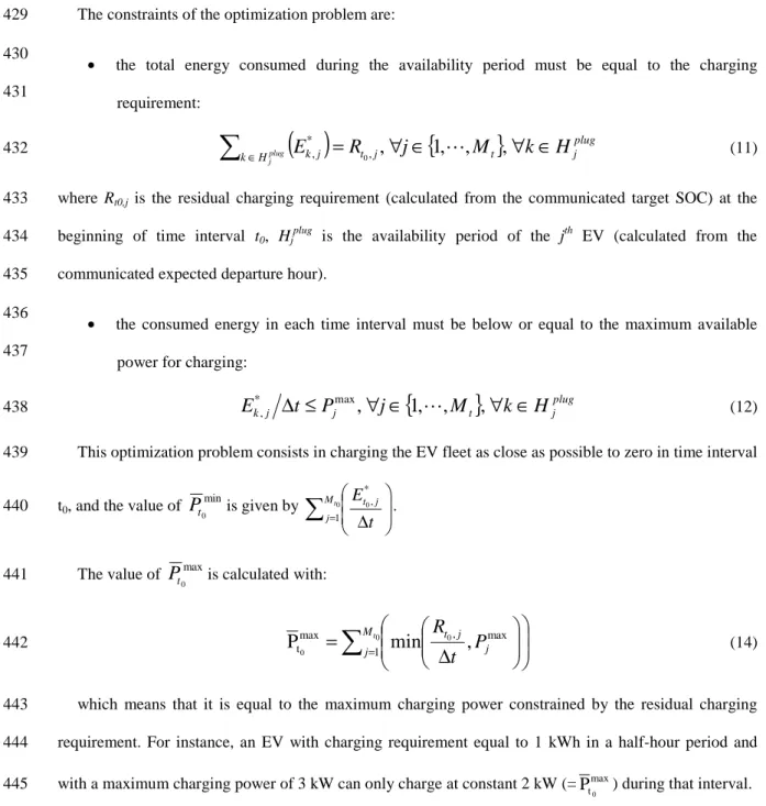
The constraints of the optimization problem are:

429

• the total energy consumed during the availability period must be equal to the charging 430

requirement:

431

( )

{

}

H

k plug

E

R j M k H

j

= ∀ ∈ ∀ ∈

∑

^{, 1 , , ,}

*

, ₀

⋯

432

where R_t0,j is the residual charging requirement (calculated from the communicated target SOC) at the 433

beginning of time interval t₀, H_j^plug is the availability period of the j^th EV (calculated from the 434

communicated expected departure hour).

435

• the consumed energy in each time interval must be below or equal to the maximum available 436

power for charging:

437

{

}

j j

k

t P j M k H

E

∆ ≤

, ∀ ∈ 1 , ⋯ , , ∀ ∈

438

This optimization problem consists in charging the EV fleet as close as possible to zero in time interval 439

t₀, and the value of ^min

t0

P

∑











∆

0 0

1

*

t , M j

j t

t E . 440

The value of ^max

t0

P

441

∑

_ ^





 





 



 



=

∆

0 1

, max max

t

min ,

P

P

t R

(14) 442

which means that it is equal to the maximum charging power constrained by the residual charging 443

requirement. For instance, an EV with charging requirement equal to 1 kWh in a half-hour period and 444

with a maximum charging power of 3 kW can only charge at constant 2 kW (= _t^max

P0 ) during that interval.

445

These two variables, together with the accepted energy bid (E_t0), are used to define the operating 446

point. Figure 4 depicts three situations that may occur in terms of energy bid value and the variables 447

required to calculate the EV fleet operating point.

448

Figure 4: Variables required to redefine the operating point of the EV fleet.

In situation (a), the accepted energy bid is within the minimum and maximum consumption power 449

limits. In order to guarantee full availability of the reserve power, the operating point should be within 450

two limits: upper power limit that guarantees full availability of downward reserve power in time interval 451

t₀ (P_t0^upper =P_t0^max −P_t0^down), and lower power limit that guarantees full availability of upward reserve 452

power (P_t0^lower =P_t0^min+P_t^up₀ ). Depending on the accepted energy bid value, the following can occur:

453

• if P_t^upper P_t^lower

0

0 ≥ (any operating point between P_t^lower

0 and P_t^upper

0 allows full availability of the 454

reserve, thus it is selected the closest point to the energy bid) 455

if

^E

^{∆ t ∈} [ ^P

, ^P

] ^{⇒ P} '

^{= E}

^{∆ t}

456

if

P

E

t P

P

0 0 0

0

> ∆ ⇒ ' =

P

0 since 457

it is the closest point to the energy bid) 458

if

P

E

t P

P

0 0 0

0

< ∆ ⇒ ' =

P

0 since 459

it is the closest point to the energy bid) 460

• if P_t0^upper<P_t0^lower,P'_t0=E_t0 ∆t (any change in the operating point value would increase the 461

reserve availability in one direction, at the cost of the other direction; the choice is to maintain 462

the operating point equal to the energy bid value) 463

In situation (b), the accepted energy bid is below the minimum consumption power level. The 464

operating point is defined as follows:

465

• if P_t^upper P_t^lower P_t P_t^lower

0 0 0

0 ≥ ⇒ ' = (the operating point is made equal to P_t^lower

0 since it is the 466

closest point to the energy bid);

467

• if P_t0^upper<P_t0^lower,P'_t0=min

(

)

in both directions; if P_t^upper

0 is greater than ^min

t0

P , it is not possible to offer upward reserve power 469

and the operating point is made equal to ^min

t0

P ; if it is lower, the operating point is made equal to 470

upper

P

0 and it is possible to offer upward reserve between this point and ^min

t0

P ^).

471

In situation (c), the accepted energy bid is greater than the maximum consumption power level. The 472

operating point is defined as follows:

473

• if P_t^upper P_t^lower P_t P_t^upper

0 0 0

0 ≥ ⇒ ' = (the operating point is made equal to P_t^upper

0 since it is the 474

closest point to the energy bid);

475

• if P_t0^upper<P_t0^lower,P'_t0=min

(

)

in both directions; if P_t^lower

0 is greater than ^max

t0

P , it is not possible to offer downward reserve 477

power and the operating point is made equal to ^max

t0

P ; if it is lower, the operating point is made 478