Sizing and Integration of an Electric Propulsion System for a VTOL UAV

I am very grateful to my parents for the emotional encouragement and financial support throughout my academic journey. Afzal Suleman, for the opportunity he gave me as well as for the support during this trip in Canada.

Nomenclature

Introduction

• State of the Art
• Motivation
• Project Overview and Requirements
• Objectives
• Thesis Outline

Therefore, the two main components of the propulsion system - the propeller and the engine - determine the overall efficiency of the system. The purpose of this thesis is to size the propulsion system for VTOL and forward flight of four scaled-down prototype UAVs.

Theoretical Background

Propeller Design

• Corke’s Propeller Design for Cruise
• Vortex Theory of Screw Propellers
• Propeller Momentum Theory

In the selection process, equation 2.1 was used to estimate efficiency [78]. where T is the thrust required in N, V ​​is the speed in m/s, P is the power required from the propeller in W and pi is the propeller efficiency. 2.2) Equation 2.2 relates the blade impact speed to the residual ones, where ω is the blade rotation speed and d is the radial coordinate. Knowing the 2D drag of the blade section, Cd and lift, Cl, the coefficients as well as the chord, cb, differential thrust and section torque can be calculated, as shown in equations 2.3 and 2.4. CdcosεB+ClsinεB) (2.4).

Visin(εi+ε∞)]2+ [Vicos(εi+ε∞)]2 (2.6) The circulation,Γ, can be calculated by the Prandtl tip loss factor,f, where βr is the aerodynamic pitch angle at the tip of the blade, combined with Goldstein's ratio between Vθi and the cross section turnover. Considering the speed upstream of the propeller is given by V∞+Vi, the free stream speed and the induced speed, respectively, the speed downstream of the propeller Vd can be obtained from. By substituting Equation 2.13 into Equation 2.12, the required power can be calculated as a function of thrust and freestream speed.

Computational Fluid Dynamics (CFD)

• Frozen Rotor Model
• Mixing Plane Model
• Transient Rotor-Stator Model
• Turbulence Model - Shear Stress Transport
• Finite Volume

This method is the simplest steady-state model and requires 50x less computational effort than the sliding mesh model, with the ability to calculate the flow properties for rotor and stator almost independently [86]. The interface of the two domains uses an arbitrary mesh interface (AMI), which projects patches from one geometry into the other, making the values ​​the same on both sides. Shear stress transport (SST) is a two-equation eddy viscosity model that uses k-ω formulation for the inner parts of the boundary layer, and switches to a k behavior in the free stream.

This Reynolds-averaged Navier-Stokes method accounts for the transfer of the main turbulent shear stress by assuming that the turbulent boundary layer shear stress is proportional to the turbulent kinetic energy [93] [94] . It requires the discretization of the geometric domain into a non-overlapping finite volume, the PDEs are then converted to algebraic equations by integration over the discrete volume and solved to obtain the values ​​of the dependent variable for each quantity. This is a strictly conservative approach that can be formulated with unstructured polygon meshes as well as with different boundary conditions, since the variables are evaluated at the centers of the volume elements [95].

Flight Dynamic Modeling

• Dynamics Model
• State Space Representation
• Control

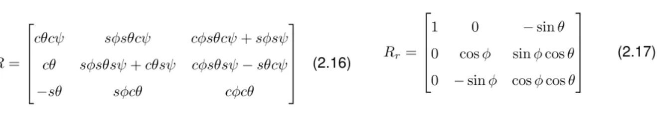
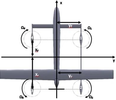
To derive the dynamics equations, the relative position of the rotors in the body frame must be defined. The state vector determines the linear and angular velocity of the UAV and its position and orientation. 2.23). In order to verify the validity of the previously set assumptions and to confirm the accuracy of the mathematical model, a closed-loop controller was derived using PID controllers [105].

The proportional component of the PID controller has the greatest influence, changing the output proportionally to the error. The integral side of the PID is responsible for the speed of response, controlled by the integral constant, KI. Finally, the derivative control mode is responsible for the rate of change of the error, which makes it ineffective with continuous errors.

Propulsion System Sizing

• VTOL Parametric Studies
• Power estimations
• Configuration Definition
• Propulsion System Selection
• VTOL System Selection and Validation
• Forward-Flight Selection and Validation
• Power Distribution and Consumption
• Propulsion System Mass Estimation
• Rotor Coverage

The choice of propulsion system is divided into two categories: VTOL and forward flight. The selection of the motor-propeller combination for the VTOL system was done through a survey of the available options in the market while respecting the project requirements. This model was used to both validate the choice for configuration one, as well as to ensure forward flight performance of the remaining configurations.

To do this, an assessment of the power required for cruising and flight was carried out. The mass of the propulsion system can be divided into two main contributors: the propulsion components and the battery. On the other hand, applying this battery allocation to other configurations would result in a decrease in total range - compared to that shown in Table 3.14 -, increasing the power available for other mission segments.

Static Experimental Tests

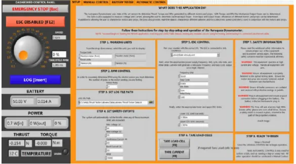
• Test Bench Set Up and Experimental Procedure
• Experimental Results
• Thrust vs Throttle
• Thrust vs Power
• Rotor Coverage Experimental Results
• Data Treatment and Results
• Motor Constants

The results were processed with a MATLAB®script, averaging the data of the different logs and the thrust and torque values ​​of the taring with those obtained for 0% throttle. Since the avionics team determined that the controller would not function properly at a T/W ratio of 1.29, making 1.3 the bare minimum, the additional available thrust may come as a benefit. With the power required for the different segments of the VTOL mission, a new estimate for battery mass can be performed to obtain a more accurate prediction of propulsion system mass.

The method for calculating the covered area based on the height of the plate is shown in figure 4.6. 5 The data for a 76% covered area at 200% distance was omitted because of its clear contradiction with the remaining results. This constant was also derived from experimental data by calculating the slope of the trend line of the torque ratio with the square of propeller rotation.

Flight Dynamic Modeling

• Quadrotor Dynamics
• Propulsive Forces and Moments
• Aerodynamic Forces and Moments
• Linearization
• Mathematical Model
• Simulink ® Model
• Model Description
• Controller Tuning
• Results
• Longitudinal Dynamics
• Lateral Dynamics
• Configuration Comparison
• Tri-rotor Dynamics

Furthermore, adapting the UAV's motion to a simple multicopter, eliminating the fixed-wing flight mode, can reduce the aerodynamic effects of drag in the multiple directions as well as the resulting moments. As for the fuselage drag coefficient Cdf, present in equations 5.6 and 5.7, it was approximated as the cylinder drag coefficient. 2ρ(−CdwSwdw+CdcScdc+ 0.5CdfSfdf)w2 (5.8) The moment in the vertical direction - given by equation 5.9 - was calculated by assuming a uniform distribution of the resistance along the hull in the lateral direction, applied to the geometric center.

In order to achieve a stable model that does not oscillate unnecessarily, but has a controlled and fast response, it is necessary to tune the gains of the proportional controllers and those of the PID controllers. The time to reach 90% of the requirement is similar to the previous example, it requires a higher speed - -4m/s. Shown here is a comparison of the behavior of configurations two and three with respect to the curves obtained for configuration one.

Flight Testing

Flight Test Preparations

Once all the connections were made and the propellers were attached, all that was missing was the battery to complete the UAV's propulsion system. All fixed-wing actuators were set to zero degrees and the pusher propeller was aligned with the rudder to avoid interference during the VTOL flights.

Flight Tests

• Hover Power Consumption

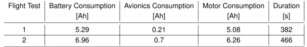
In the absence of this device, the current consumption of each motor was unknown and had to be estimated from the battery consumption. Knowing the total capacity consumed by the engines and the duration of the flight, the average current passing to each engine can be calculated, as shown in equation 6.1. F light Duration = 4×M otor Current⇒M otor Current= Capacity consumption 4×F light Duration (6.1) The average current was multiplied by the average voltage per test to calculate power consumption for each flight test.

When comparing the average throttle position at which the engines were operating with the expected throttle position there is also a discrepancy. The estimated hover throttle from the static tests was lower than the setting required during the flight tests. In terms of thrust, the 76% throttle setting can be associated with a force of 78 N, which represents a hover condition for a 7.95 kg UAV.

Conclusions

Summary

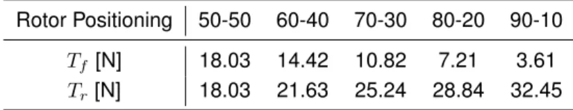
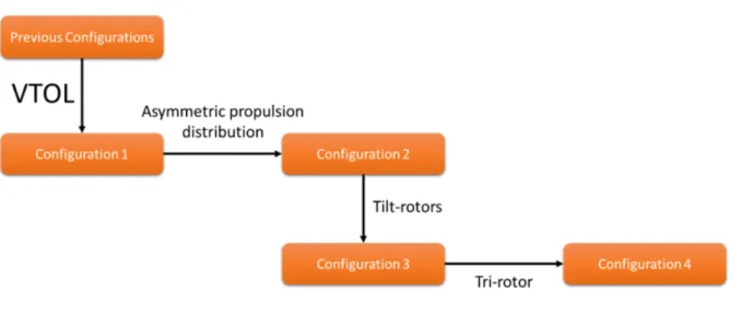
Configuration one adds a VTOL system to the previous UAVs developed for the mission, with a pusher to complete the lift-and-cruise architecture; In comparison, configuration two has the same architecture but an asymmetric thrust distribution, with the rear rotors producing 80% of the thrust required during VTOL. The VTOL system selection of all configurations was performed with experimental data from manufacturer websites, and compared with the results of a vortex theory model for validation. Finally, configurations three and four were adjusted with the vortex theory model by adjusting the required parameters.

Having sized all the configurations, their performance was evaluated, studying the total power installed as well as the power available for forward flight, the total mass of the system and its power requirements. In terms of installed power, configuration four performs the mission with the least excess power, at over 73%. At cruise, configurations three and four are the most efficient, with 97 and 97.5% of the power of configuration one, while configuration two has a penalty of over 20%.

Achievements

When evaluating mass, configurations three and four stand out, having both the least total energy requirements and the lightest component mass. The increased performance of configurations three and four was hampered by having rotors partially covered, which required a minimum distance between surfaces to obtain a satisfactory net power. With both the CFD simulations and the experimental results, the asymptotic behavior of the curves was proven, concluding that for the given cases there is a minimum relative required distance of half a radius, with a penalty of 1 % in total mass - including battery for one mission and all components - for a distance of 75% of the propeller radius; this still makes them the lightest, yet not the most energy efficient.

Finally, a dynamic model was developed for configurations one through three, concluding that all simulated configurations are controllable and stable, with virtually no differences in behavior for the same desired posture. The flight test data concluded that the system consumed significantly - 20% - more power than estimated from static testing. Although this discrepancy is significant, it can be explained by the approximations made in ignoring the maneuvers performed in flight and the additional power required to do so.

Future Work

Bibliography

Preliminary sizing, flight test and performance analysis of a small tri-rotor VTOL and fixed-wing UAV. A Critical Review of Unmanned Aerial Vehicle Power Supply and Energy Management: Solutions, Strategies, and Prospects. Implementation of a vane element momentum model on a polar grid and its influence on aeroelastic loading.

Analysis of power losses in gear transmissions - measurements and CFD calculations based on open source codes. Sliding mesh algorithm for CFD analysis of helicopter-fuselage rotor aerodynamics. International Journal for Numerical Methods in Fluids.