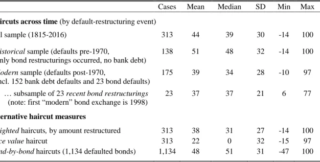
We are the first to quantify foreign sovereign bond returns with long-term price data, despite the fact that this is one of the largest and oldest asset classes worldwide.8 The possible explanation is the limitations of data. Haircut 𝐻𝐻𝑡𝑡𝑖𝑖in restructuring 𝑖𝑖 at time 𝑡𝑡 is calculated by comparing the net present value (NPV) of the contractual payment flows of the new debt issued in the restructuring with the old debt in default of NPV. For a meaningful comparison, the same discount rate should be applied to calculate the NPV of the new bonds and the old (defensive) bonds.
Both old and new bonds face the risk of another default in the future, and they both benefit from the debt relief effect of the restructuring. To choose the discount rate 𝑟𝑟𝑡𝑡𝑖𝑖, we follow Sturzenegger and Zettelmeyer (2006) and Cruces and Trebesch (2013) and use the "exit yield", which is the secondary market rate of the new bonds that start trading after the restructuring. The size of the circles represent the inflation-adjusted debt amounts affected by the restructurings (in real 2009 US$).
Note: Some of the haircuts shown are negative, but these are only 10 events and they mostly occur at the beginning of debt problems (see footnote 23). For example, Lenin canceled all foreign debt in the wake of the Communist Revolution in 1917.

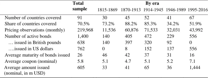
Sovereign bond returns, 1815-2016
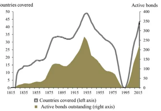
In the first half of the 19th century (after Waterloo), less than 20 countries traded sovereign bonds in London. After World War I, New York joins London as the second dominant financial center of the world, and our sample continues to grow, reaching a first peak in the late 1920s. By definition, all bonds in the sample are denominated in either GBP or USD, so we need historical inflation data for the UK and the US to calculate real returns.
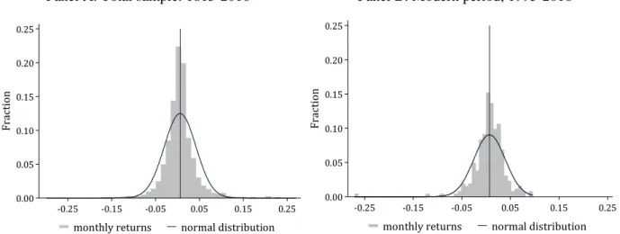
More precisely, we calculate 𝑅𝑅𝑃𝑃𝑖𝑖,𝑗𝑗,𝑡𝑡 = 𝑅𝑅𝑖𝑖,𝑗𝑗, 𝑠𝑠,𝑡𝑡, where 𝑅𝑅𝑃𝑃𝑖𝑖,𝑗𝑗,𝑡 is the risk-free rate, denominated in the same currency as the bond. As a result, the number of countries with actively traded bonds drops to less than 10 in the 1980s, making the global portfolio unrepresentative. Nominal returns exceed real returns in the full sample, but this is driven by the post-World War I period.
In the modern (after 1995) period, the share of bonds with negative returns is much smaller than in the historical sample (Panel B). Returns by country or group are averaged across all active bonds in the subsample and weighted by volume, similar to global portfolio construction. Serial defaulters show higher excess returns in the full sample and in most models, except in the interwar years, when central government bonds outperform.
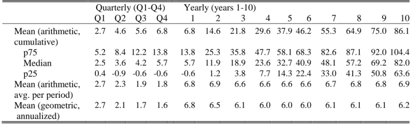
The typical serial default (marked in red) has average annual returns in the 5-10% range and a standard deviation of returns above 20%.
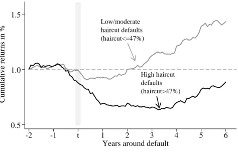
Bond performance around debt crises: returns, defaults and haircuts
The bold black line shows the average across all bonds in the global portfolio, while the dashed gray lines show the upper and lower quartiles. Almost all defaults in this bottom quartile occur in the historical period (before WW2), including the defaults that took decades to settle. Moving beyond default episodes, Figure 11 compares annual average real ex-post yields on government bonds with the annual average haircuts, both in the historical bond period and in the modern period.
During the historical period, the average return on our global portfolio of external bonds was 6.4%. Note: This figure shows average ex-post real returns on our global portfolio of foreign currency government bonds and compares it to the size of the haircuts, both calculated as annual averages. In this section, we compare the returns on external government bonds from our new database with the returns for other major asset classes traded on the UK and US capital markets.
As in the previous analysis, we use a global portfolio time series of returns on all active foreign currency sovereign bonds in the sample, weighted by debt amounts. However, as an alternative, we also report excess returns over long-term UK or US bonds, which has been our approach so far, but is less standard in the literature comparing asset classes. Notes: The table shows average annual actuarial returns of our global portfolio of external sovereign bonds as well as for other asset classes traded in London and New York.
The main insight from Figure 12 and Table 7 is that, over the two centuries under study, a global portfolio of external sovereign bonds exhibits favorable risk-return properties relative to other financial assets. Foreign sovereign bonds also show a high Sharpe ratio, on a par with US equities, and exceeding that of UK equities, US corporate bonds and US or UK government bonds the Great. Foreign sovereign bonds show higher cumulative returns than stocks in two of the three periods (through the end of the third year).
During the 2008 financial crisis, external government bonds delivered worse returns than US bonds at the height of the crisis, but subsequently performed much better. Taken together, these findings suggest that peripheral government bonds can provide insurance against major shocks to the financial center. The high average coupon payments on external government bonds help stabilize total returns when prices are volatile.
Conclusion
On the link between the credit distribution puzzle and the equity premium puzzle, Review of Financial Studies. Country Debt Development and Economic Performance, Volume 1: The International Financial System, University of Chicago Press, Chicago & London, pp.
Appendix to “Sovereign Bonds since Waterloo”
In case the date of partial coupon payments is missing, we assume that the debtor paid on the specified coupon date (original due date). Where 𝑃𝑃𝑝𝑝𝑝𝑝𝑎𝑎 𝑏𝑏𝑝𝑝𝑛𝑛𝑎𝑎, Indices are indexed by 1 at the beginning of the period (January of the year).
We start with the modern part of the sample and use data for 187 restructuring events covered in the most recent update of Cruces and Trebesch (2013). A further seven cases resulted from the disintegration and dissolution of the Ottoman Empire (for details see the section on state divisions below). In the Brazil example above, we calculate an average haircut of the 1943 and 1946 agreements and assign the year 1943.
The second approach compares the present value of the debt payments for the new instruments and compares it to the nominal value of the old debt. More specifically, in our historical sample, delinquent interest averages 34% of the old outstanding principal. Bond buybacks: About 50% of the bonds in the sample of historical debt restructurings contain repurchase clauses.
These golden clauses are not valued when calculating haircuts, as they were not legally binding, especially after the repeal of the golden clause in Britain in 1931 and in the US in 1933. Timing: The month of the final agreement serves as ' a baseline date to calculate cash flow streams. The successor states agreed to divide the debt in 1832 in the wake of the partition.6.
Therefore, selective agreements of the same debtor country but different creditor groups were coded separately in the raw data set. However, as explained above, we also combine examples of the same default in the main document and analysis. In these cases, let's assume a cumulative sinking fund amortization plan (comparable to an annuity scheme), as this was the most common approach in the 19th and early 20th centuries.
In particular, we do not need to make assumptions about future interest rates, as in the case of floating rate loans that were dominant in the sovereign debt markets of the 1970s or 1980s. Holdouts: The haircut calculations in this paper aim to capture the loss of the average creditor who participates in the restructuring.