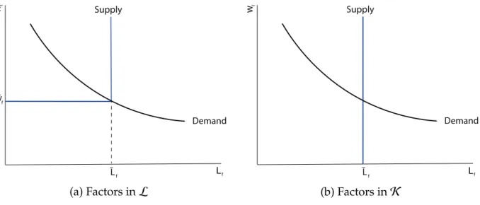
5 We withdraw from investing in the main part of the paper to keep the outline manageable. The other possibility is that wf = w¯f and the use of the factor is less than potential Lf ≤ L¯f.
Comparative Statics
This type of supply-driven underemployment would occur even in the absence of downward nominal wage rigidities. On the other hand, the pandemic may reduce households' willingness to consume in the present relative to the future: for given prices and income, households may choose to consume less during the epidemic and more afterwards.
Input-Output Definitions
The inverse Leontief matrix Ψ records direct and indirect exposures through supply chains in the production network. We define the weight Domarλi of production, to be its share of sales as a share of GDP λi ≡ piyi.
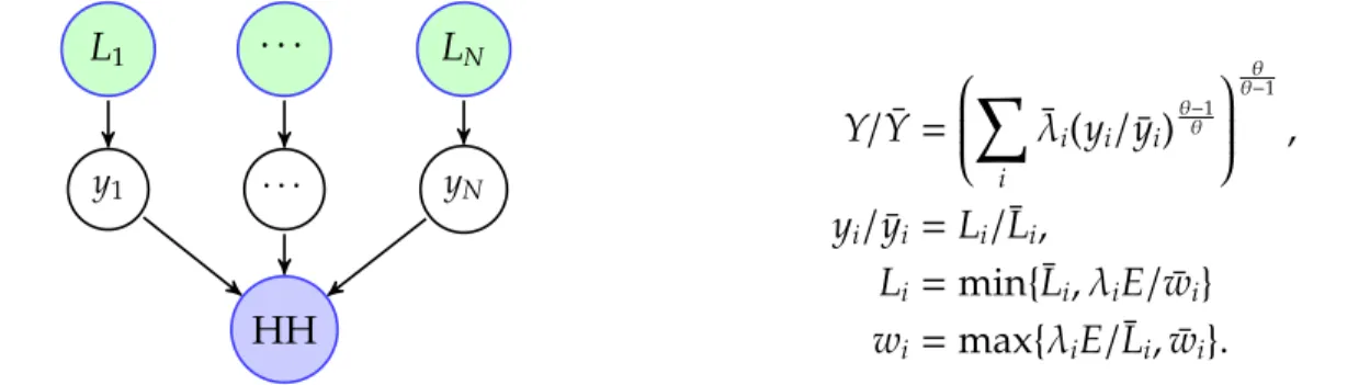
Nested-CES Economies
3 Local Comparative Statics
- Euler Equations
- Aggregation Equation for Output
- Propagation Equations for Shares, Prices, and Factor Employment
- A (Somewhat) Universal Example
Summing all supply-constrained factors and solving the resulting linear equation gives changes in total spending on supply-constrained factors. This can be used to infer average changes in employment in the demand-constrained factors.
4 A Benchmark with Simple Network Su ffi cient Statistics
- Global Su ffi cient Statistics
- Lattice Structure and Global Comparative Statics
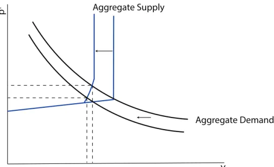
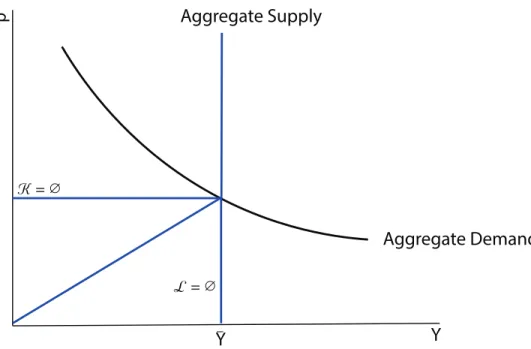
- AS-AD Representation
- Keynesian Amplification and Complementarities
- Keynesian Amplification and Shock Heterogeneity
- Interaction of Sectoral Supply Shocks and Aggregate Demand Shocks
- Shocks to the Sectoral Composition of Demand
- Benefits of Wage Flexibility and of Factor Reallocation
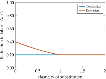
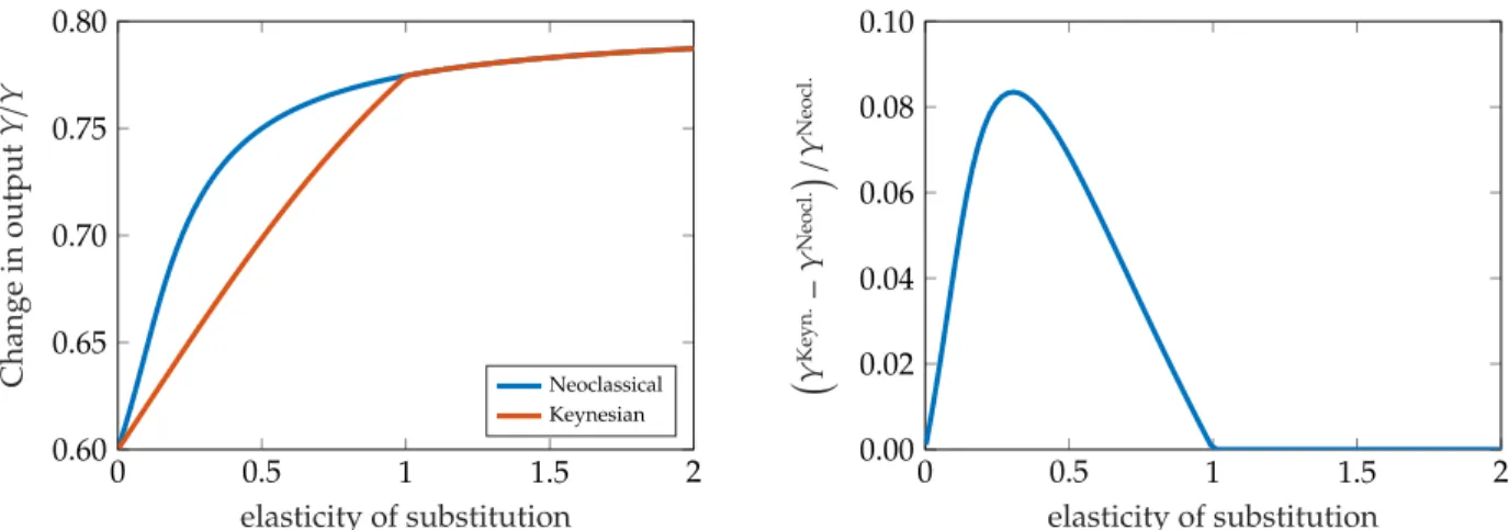
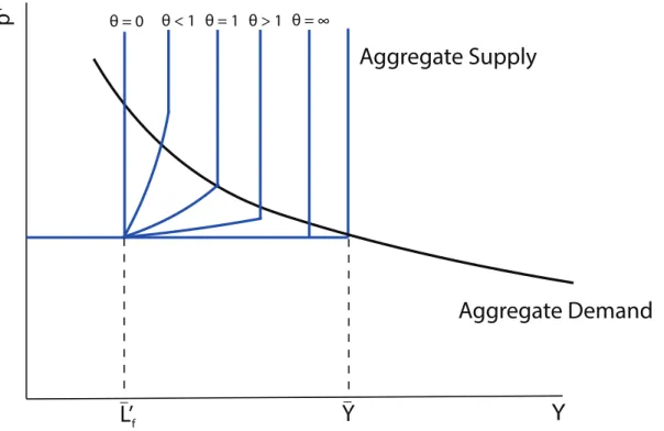
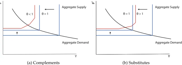
This notion is different from the Keynesian extension of negative supply shocks to factors of limited supply that is used for equation 3.3. In other words, the magnitude of Keynesian unemployment in demand-constrained factor markets decreases as a function of the elasticity of substitutionθ. In the figure, we draw a new AS curve for different values of the elasticity of substitution θ.
First, consider the case where there is only a negative supply shock due to one of the factors.
5 Quantitative Application
- Setup
- Role of Supply and Demand Shocks
- Role of Intertemporal vs. Intersectoral Shocks
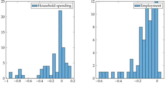
- Tightness and Slackness Across Sectors
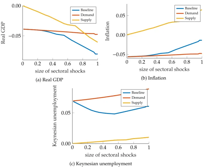
The "baseline" line includes a negative aggregate demand shock as well as sector-specific supply shocks and shocks to the sectoral composition of demand. The demand line includes a negative aggregate demand shock and shocks to the sectoral composition of demand. Intuitively, when the "magnitude of sector shock" is zero, all labor markets are slack due to the negative aggregate demand shock.
The “Baseline” line includes a negative aggregate demand shock (intertemporal shock) as well as sectoral supply shocks and shocks in the sectoral composition of demand.
6 Extension I: Credit Constraints and Household Spending
Local Comparative Statics
The key step in this extension is the determination of changes in aggregate nominal expenditure. The expectation uses factor shares in the future λ∗f for f ∈ G as probability distribution and ΛH =P. In this version of the model, there is now an endogenous aggregate demand shock, even in the absence of exogenous aggregate demand shocks, such as changes in nominal interest rates or in the desire to save.
In particular, as the income earned by factors falls, this gives a negative aggregate demand shock that causes nominal expenditure today to shrink dlogE<0.
Global Comparative Statics
In particular, sectoral supply shocks dlog ¯L < 0 and shocks in the composition of sectoral demand dlogω0 are still inflationary around equilibrium. To see this, combine (6.1) with Theorem 1, and set all other shocks to zero to get.
7 Extension II: Credit Constraints and Firm Failures
Local Comparative Statics
They provide a mechanism by which a negative demand shock, say in the composition of demand or in aggregate demand dlogζ, causes exits that are isomorphic to negative supply shocks. As in the other examples, the general lesson is that the output response, to a first order, is again given by an application of Hulten's theorem together with a reinforcement effect that depends on how the network redistributes demand and Keynesian unemployment in some factors cause. and fixed failures in some sectors.
Illustrative Example
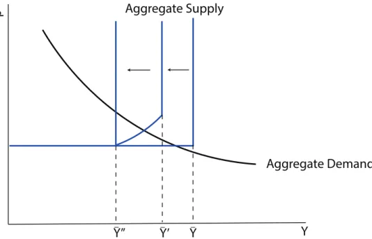
The second term captures the further indirect equilibrium reduction in output through firm failures and Keynesian unemployment in the other sectors. Sector loses demand after the exogenous closure of some of its firms, and this leads to unemployment in the sector (dlogLi <0), but no endogenous firm failures (dlogMi =dlog ¯Mi). In the Cobb-Douglas case, in response to an exogenous shutdown shock, the AS curve shifts but retains its shape.
When sectors are substitutes, Keynesian unemployment arises in the shocked sector, as the shocked sector loses revenue to other sectors.
8 Extension III: Policy
Monetary Policy
Outside of the Cobb-Douglas case, the AS curve also changes shape and there is Keynesian unemployment regardless of whether the sectors are complements or substitutes, as captured by the fact that the AD curve intersects the AS curve in the upward-sloping portion to the left. of its vertical part. The first term is the effect of a negative supply shock reinforced by nominal rigidities, exactly as in case 3.4. The term (1−λS)dlogζ is the direct effect of the stimulus on the employment of factors that limit demand.
This is because monetary stimulus increases the prices of supply-constrained factors in absolute terms and relative to those of demand-constrained factors, and since supply-constrained and demand-constrained factors are complements, it causes expenditure to shift to supply-constrained factors and away from demand-constrained factors.
Payroll Tax Cuts
In addition, we assume that the government implements a gross wage subsidy on the demand-driven factors, financed by a tax on the resulting profit. Of course, a subsidy on demand-limiting factors increases output, and the term (1−λS)dlogsD is the direct effect of the increase in employment. However, the subsidy on demand-constrained factors also lowers the price of slack sectors compared to supply-constrained sectors.
Since the factors are complementary, this means that expenditure is diverted towards supply-constraining factors and away from demand-constraining factors, reducing the effect of the wage subsidy.
Fiscal Policy
As usual, the first term is the effect of the negative supply shock for the supply-constrained sectors, amplified by the nominal rigidities. The first reason is the standard Keynesian cross-argument: an increase in government spending stimulates the income of households, which then go on to consume more. This increases nominal expenditure by dG(1−αRicardianMPCRicardian)/(1−MPC), which is higher, the higher the average marginal propensity to consume MPC and the lower the fractionαRicardian of future taxes falling on Ricardian consumers.34 Interesting enough, in the context of the pandemic, the fiscal multiplier may be lower in a partial austerity if Ricardian households have a low marginal propensity to consume because they want to delay consumption until the austerity is fully lifted.
To the extent that the government cannot fully target depressed factor markets, some government spending will end up wastefully raising the wages of supply-constrained factors rather than stimulating employment, thereby lowering the fiscal multiplier.
9 Conclusion
Intuitively, fiscal policy can shift the AD curve by changing both the size and the sectoral composition of public spending. Furthermore, fiscal multipliers are further dampened in economies with complementarities, as government spending to some extent always ends up raising wages for some supply-constrained factors, causing private spending to be redirected toward those factors and away from demand-constrained factors.
Boehm, Christoph E, Aaron Flaaen, and Nitya Pandalai-Nayar, “Input Linkages and the Transmission of Shocks: Firm-Level Evidence from the 2011 T ¯ohoku Earthquake,” Review of Economics and Statistics. Brinca, Pedro, Joao Duarte, and Miguel Faria e Castro, "Measuring Sectoral Supply and Demand Shocks during COVID-19," Technical Report 2020. Guerrieri, Veronica, Guido Lorenzoni, Ludwig Straub, and Iván Werning, "Macroeconomic Implications of COVID-19: Can Adverse Supply Shocks Cause Demand Shortages?," Technical Report, National Bureau of Economic Research 2020.
Ozdagli, Ali and Michael Weber, “Monetary Policy Through Production Networks: Evidence from the Equity Market,” Technical Report, National Bureau of Economic Research 2017.
Appendix A Additional Graph
Appendix B Investment
General local comparative statics
This follows from the fact that the nominal expenditure for each factor f is given by dlogλIf + dlogEI, where EI is the net present value of household income. However, since nominal expenditures are fixed in the future, we have dlogE∗= dlogλI∗+dlogEI =0. This allows us to write nominal expenditures for each factor as dlogλIf −dlogλI∗.
Global Comparative Statics
Appendix C Some Downward Wage Flexibility
Generalizing the Results
Illustrative Example
This reduces the shares of demand-limiting factors, creates unemployment and further reduces output through Keynesian effects. The difference between the case where wages have some downward flexibility (φ < ∞) and the case where they do not (φ = ∞) is that now the wages of the demand restraints are falling, and this mitigates the rise in unemployment and the reduction of output. However, there is also a compensating reinforcing effect: the labor supply shocks on the demand-limiting factors now also matter.
This is because these shocks now lower the wages of the demand-constraining factors, further diverting expenditure away from them due to complementarity, further reducing the employment of the factors.
Appendix D More Examples
Cobb-Douglas Economy
Of course, allowing some degree of wage flexibility can make endogenous changes to the ranges of supply and demand constraining factors, which is why we do not proceed with the comparison. In the Cobb-Douglas example, the demand shocks dlogω0 and dlogζ only propagate backward along supply chains to cause unemployment upstream. On the other hand, supply shocks dlog ¯Lf and dlogAi only spread forward along the supply chains, but do not cause unemployment downstream.
Indeed, since these shocks do not change the factor shares, supply shocks do not cause any unemployment in either factor, so these shocks do not trigger Keynesian channels.
Substitutable Supply Chains
Unlike Example 3.4, where complementarities create unemployment in non-shocked supply chains, in this example, substitutability creates unemployment within the shocked supply chain. However, there may be unemployment in 1 and/or 3 and we focus our attention on these sectors. Here the first term on the right-hand side coincides with the impact of the negative labor supply shock in the neoclassical model.
The second term on the right is negative and represents the additional fall in output through the Keynesian channel via increases in unemployment in sector 3.