DOI 10.1007/s11134-012-9316-8
The single-server scheduling problem with convex costs
Carlos F. Bispo
Received: 3 January 2011 / Revised: 30 April 2012
© Springer Science+Business Media, LLC 2012
Abstract Being probably one of the oldest decision problems in queuing theory, the single-server scheduling problem continues to be a challenging one. The original for- mulations considered linear costs, and the resulting policy is puzzling in many ways.
The main one is that, either for preemptive or nonpreemptive problems, it results in a priority ordering of the different classes of customers being served that is insensitive to the individual load each class imposes on the server and insensitive to the overall load the server experiences. This policy is known as thecμ-rule.
We claim and show that for convex costs, the optimal policy depends on the in- dividual loads. Therefore, there is a need for an alternative generalization of the cμ-rule. The main feature of our generalization consists on first-order differences of the single stage cost function, rather than on its derivatives. The resulting policy is able to reach near optimal performances and is a function of the individual loads.
Keywords Scheduling·Production control·Queuing systems·Dynamic priorities·cμ-Rule
Mathematics Subject Classification 90B22·90C39·90C40
1 Introduction
The setting for the problem we address consists of a single server that can process different classes of customers, which arrive from the outside world and queue up in front of it, waiting for service. There will be one queue per class, and each queue is served on a first-come-first-serve basis. The arrival process is noncontrollable, and
C.F. Bispo (
)Instituto de Sistemas e Robótica, Instituto Superior Técnico, Av. Rovisco Pais, 2049-001 Lisbon, Portugal
e-mail:cfb@isr.ist.utl.pt
each class requires different processing times that, in general, are assumed random and a priori unknown to the server. Whenever the server concludes a service, it will have to decide which of the classes to serve next, out of the ones which have cus- tomers present. It is assumed that there is a cost associated with each queue that is proportional to the number of customers in that queue or, conversely, proportional to the waiting time of the customers. So, the growing of the queues constitutes the incentive for the server to work.
In general, considering that there arexi(t )customers of classifori=1,2, . . . , K, at the time instantt, the single-stage cost for classican be defined to beCi:N→R such thatCi(xi)is nondecreasing inx and convex forx∈R. Here we dropped the explicit time dependence for convenience. Furthermore, we will be interested in the cases where these functions are convex. For a finite-time problem, under some de- cision policy, one may take the expected value over all possible trajectories of the integral over time of the single-stage cost functions sum for all classes. If the length of the trajectory is unbounded, one may choose to take a series of fixed-length time average of that expected integral with growing length, i.e., infinite-horizon average costs, or take the expected integral of the discounted sum of the single-stage costs, i.e., infinite-horizon discounted costs. That is,
Tlim→∞
1 TE
T
0
C(x) dx
(1) or
E ∞
0
e−βtC(x) dx
. (2)
An optimal policy will be the set of decisions, a function of the k-tuple (x1, x2, . . . , xk)at any decision point, that for each of the above cases will achieve the minimal cost.
If the service can be preempted and later resumed for any class, there will be two decision points, the completion of a service and the occurrence of an arrival. For the nonpreemptive case, only a service conclusion is a decision point. The only exception to this is when an arrival occurs while the server is idle because, prior to the arrival and upon conclusion of the last service, there were no customers waiting for service.
We also focus on the case where there is no cost associated with activating the server, i.e., no warm up cost, and no cost associated with switching from a class to another, i.e., no set up, or change over, cost.
The classic approach to this problem assumed that the single-stage costs are lin- ear, e.g., Ci(xi)=cixi. When such is the case, for both infinite cost versions, in general, the optimal policy is known as thecμ-rule. That is, assuming that the aver- age processing time for classiis 1/μi, the optimal policy is such that at any decision point, the server will engage service with the head of the nonempty queue of the class which possesses the highest value ofciμi. An easy way to interpret intuitively this rule is to consider that if all the processing rates are the same, priority should be given to the most costly queue, or to consider that if all the single-stage costs are the same, priority should be awarded to the queue with the shortest average processing time.
The oldest known reference to a version of this problem dates back to 1956. It is considered that Smith [19] was the first to suggest the optimality of thecμ-rule. His setting was deterministic and static. That is, the processing times are fixed for each class (deterministic), and all the customers are present at time 0, and no arrivals are allowed after that (static). Outside the queuing theory community, in the scheduling theory community, this is also referred to as the WSPT (Weighted Shortest Process- ing Time) rule. Later, Cox and Smith [8] showed the cμ-rule to be optimal for a stochastic, dynamic environment with arbitrary time horizon. Their setting was that of a multiclassM/G/1 queue. They considered both preemptive and nonpreemp- tive cases. Naturally, it came with not much surprise that this rule is also optimal for stochastic and static settings; Pinedo [17] and Righter [18] are examples where such result can be found.
The amount of extensions and variants of the problem that have been considered after Cox and Smith is quite significant. For more references on related work, we refer the reader to the literature review presented in [20]. We only consider a sample of the ones that focus on the simpler problem, i.e., no feedback for instance. Out of those, Harrison [13] considered a multiclassM/G/1 with the added feature that there are also rewards for each service completion. His policy is slightly more complex than thecμ-rule, as hisβ-optimal,β being the discount parameter of a continuous-time problem, specifies a priority ranking also, but some classes may never be served.
The ranking is a function ofβ, which is not the case of the original problem. Also, the ranking is not defined by the simplecμ-rule. We believe that these differences are explained by the inclusion of rewards, which distorts the original problem sig- nificantly. For the case of discrete-time problems, one example of optimality of the cμ-rule was presented by Buyukkoc, Varaiya, and Walrand [6] for multiclass sys- tems under arbitrary arrival processes, geometric service times, and preemptive disci- pline. This followed the work of Baras, Dorsey, and Makowski [4], which established the optimality of thecμ-rule, considering only two classes of customers, with arbi- trary arrival processes and service completions generated by independent Bernoulli streams.
One of the most intriguing features of this problem is the fact that the arrival rates play no role on the optimal policy structure in all the above-mentioned variants under linear costs. Defining asλi the average arrival rate for classiand defining as indi- vidual load of classi the ratioλi/μi, the fact that each class may have a higher or lower individual load is of no consequence on the optimal policy. This raises, in some sense, an issue of fairness. Suppose that there are only two classes of customers and the lower priority class has an individual load close to 10 %, sayλ1=1 andμ1=10, while the high priority class has an individual load close to 90 % (heavy traffic), say λ2=90 andμ2=100, for instance costs are similar, but processing rates are differ- ent. A customer of the nonpriority class may see many customers of the priority class being served first, despite the fact that they may have arrived after. A consequence of this is a high variance of the waiting time for the nonpriority customers. Naturally, the nonpriority customers have more difficulty estimating when will they leave the system, and, while waiting, each arrival they see occurring for the priority queue has to be a source of disappointment. The linear cost model tells us that the marginal pa- tience of the customers is always the same no matter how much time they have been
waiting. That is, the willingness to wait an extra time unit is the same after a handful of services that it was upon arrival. Whoever has stood in a nonpriority queue knows that this is not true.
One natural consequence of customer’s impatience is a high abandonment rate, or worse. Naturally, one could argue that the abandonment behavior could be incorpo- rated in the model and the appropriate policy could be afterwards derived. Although our paper will take a different approach by considering convex costs, an instance of work incorporating abandonments is [14], where an asymptotically optimal policy is derived. More recent examples of asymptotically optimal policies where abandon- ment is included in the model are presented in [2] and [3]. Optimal policies are also studied in [3], e.g., a two-user optimal policy is given, where indices are not separa- ble anymore, and in [11], where a sufficient condition for optimality of thecμ-rule is given.
Another interesting feature of the linear cost problem is the fact that the optimal policy,cμ-rule, is intrinsically myopic. That is, what appears to be the best short- term decision agrees with the long-term best decision. Associated with this, given its simple structure, it appears that the processing rate should be multiplied by the derivative of the cost function when the single-stage costs are linear.
The first work on this problem that addresses the concern of fairness is that of Van Mieghem [20], who considers the single-stage cost to be a convex function of the delay for multiclass single-server systems. Then, he proposes to use the generalized cμ-rule, wherecis replaced by the first derivative with respect to delay of the single- stage cost function. By performing a heavy traffic analysis, the author shows that this generalized rule is asymptotically optimal, in the sense that the cost achieved under this policy approaches the cost of the optimal policy as the sum of the individual loads approaches unity. Following this work, Mandelbaum and Stolyar [16] extend the analysis to a case where the single server is replaced by a pool of multiskilled servers that work in parallel, considering convex single-stage costs as functions of the individual queue lengths. They also establish the asymptotic optimality of the generalizedcμ-rule by means of conducting a heavy traffic analysis. The maximum pressure policies of [9,10] for general stochastic processing networks produce ex- actly Van Mieghem’s generalizedcμ-rule for single-server problems.
While agreeing with the inclusion of convex costs to better reflect the marginal patience of the waiting customers, we believe that there are two points on the gen- eralization that deserve further discussion. The first point concerns using the deriva- tive of the single-stage cost function to generalize thecμ-rule. Firstly, we stress that each Ci :N →R and one can construct many convex such functions which have no derivative when assuming their domain to be the set of real numbers. Second and probably the most relevant issue is that one can formulate this as a continuous- time Markov Decision Problem, assuming Poisson arrivals, exponentially distributed service times, and apply Dynamic Programming to compute the optimal policy, for instance, through a policy iteration algorithm. Given the fact that the state space is a k-tuple of integers and that through its successive iterations the algorithm only pro- duces valid state space transitions, one should wonder how would it be possible to converge to derivatives. In other words, is the simplicity of the linear costs hiding something else?
The second point concerns the fact that the individual loads are still not playing any role on the structure of the optimal or suboptimal policies, which is intriguing, to say the least. One exception to this is the work of [1,12], where the authors de- rive an index heuristic for convex costs by formulating a restless-bandit problem.
Their approach considers preemptive service [1] or nonpreemptive service [12], and the resulting index is a function of the individual arrival rates. In both cases it only considers the cost gain of reducing the queue length of the served class.
It is the purpose of the work presented here to further our knowledge on this prob- lem, and to accomplish this, we will show that the optimal policy does depend on the individual loads and that a better generalization of thecμ-rule relies on first-order differences of the single-stage cost function. Our generalization includes also the in- fluence of cost increases when a queue gets an extra customer while being served, not just the cost reduction due to a departing customer, as in [1,12]. On this last finding, note that for linear costs, they are exactly the same, thus justifying that the linear costs may be hiding a more interesting feature.
Naturally, these findings will have to be reconciled with [10,16,20], as our work does not question the validity of the results there reported. In fact, the asymptotical optimality of their generalizedcμ-rule, which we will term as the Gcμ-rule, does not conflict with the fact that, in general, we get costs no further from the optimal costs with our proposed suboptimal policies and even achieve better results than the Gcμ-rule.
In what follows, we will first formulate an MDP for a two-class single server with convex single-stage costs in Sect.2. The restriction to two classes is done due to the fact that we intend to numerically compute the optimal policy and do not want to be overwhelmed by the curse of dimensionality [5]. Also, in Sect.2, we will address the issue of state representation of MDPs that constitutes a generalization of the com- monly accepted standard form. Then, in Sect.3, we establish a set of very interesting results for particular instances of the single-server scheduling problem that will help us identifying how should thecμ-rule be generalized. These results are valid per se, as some of the systems considered can occur in real life. Following this, in Sect.4, we present some numerical examples that illustrate that the optimal policy is a function of the individual loads. Inspired by the results of Sect.3, we propose a generalization of thecμ-rule and present numerical data to support our claim that it is possible to have a better generalization than the existing ones. Finally, we conclude in Sect.5, establishing a bridge between our work and previous work, and pointing directions for further research.
2 The model
To avoid excessive clutter, we are going to restrict the derivation to a system serv- ing only two classes of customers. The extension of the model to more queues is straightforward. Letλi be the average arrival rate for classifori=1,2, and assume that customers arrive according to independent Poisson processes. The processing requirements of each customer are assumed to be statistically the same within each class, with service times being exponentially distributed with mean 1/μi. Each ser- vice duration is independent of previous service durations and independent of the
number of customers waiting in the system. Once started, a service may or may not be preempted and later resumed with no penalty. We will address both cases where preemption is and is not allowed, because there are some issues worth discussion concerning the later. Upon conclusion of a service, the customer being served leaves the system.
We define asX(t )= [x1(t ) x2(t )]the amount of customers of both classes present in the system at timet. Given that there is only one server, it may be the case that either a customer of class 1 or of class 2 is being served whenX(t )is in the positive quadrant, while all the others are waiting. Also, we assume idleness as a possible decision for the server, although it will be seen later that the server never chooses to remain idle if there is at least one customer in one of the two queues. Given the fact that customers in the same queue are undistinguishable, each queue is served by the order of their arrival to the system, although customers of a given queue may be served prior to customers of the other queue that arrived earlier to the system.
Our state description will also have to include the state of the server when we consider the no-preemption model. Therefore, we define asZ(t )= [X(t ) y(t )]the state of the system, wherey(t )∈ {0,1,2}is the server state at timet. Ify(t )=0, the server is idle, or serving a customer of classiify(t )=i.
We will consider an infinite-horizon discounted cost criterion with discount pa- rameterβ >0 and will be interested in obtaining a stationary Markov policy. A pol- icy is defined as a function that maps the state into one of the three options for the server state. If the decision is not a function of the time instant, the policy is said to be stationary.
With the instantaneous cost rate defined earlier, we can define the expected present value of future costs, under a policyπ, as follows:
J
Z(0), π
=EπZ(0) ∞
0
e−βtC Z(t )
dt
, (3)
whereEZ(0)π {·}denotes the expectation with respect to the probability distribution of the path space ofZ that corresponds to initial stateZ(0)and control policyπ, and C(Z(t ))=C1(x1(t ))+C2(x2(t )). We then define the value function as
V Z(0)
= inf
π∈ΠJ
Z(0), π
forZ(0)∈S, (4)
whereS defines the set of all possible states, andΠ defines the set of all station- ary policies. We will useV (X(0))in the preemptive case andV (X(0), y(0))in the nonpreemptive case. In what follows, we will first detail the preemptive case fol- lowed by the detail of the nonpreemptive case. Afterwards, we compare the equa- tions and show that the standard formulation of MDP needs to be changed to ac- commodate systems where the server state needs to be captured in the overall state description.
2.1 Detail for the preemptive case
When preemption is allowed, any service conclusion event and any arrival event con- stitute decision epochs, i.e., will trigger the decision maker. For the first type of events
the server will have to decide which of the queues to serve if both of them have cus- tomers or to remain idle. In the event of an arrival while the server is busy, it has to decide if it should switch to the class of the newly arrived customer or continue with the customer with which it has engaged previously. Under these circumstances, there is no need to explicitly include the server state for stationary policies. Given the fact that the policy produces always the same decision for the same values ofxi, knowing the queue lengths is enough to know what are the feasible transitions out of that state.
Because we are dealing with a continuous-time Markov process, we resort to the uniformization procedure to convert it into a discrete-time problem. Defining the uni- form rate asγ ≥λ1+λ2+μ1+μ2≥0,α=γ /(β+γ )and omitting the explicit time dependency to avoid an excessively cumbersome notation, the value iteration algorithm [5] for this problem becomes
Vk+1(X)= 1
β+γ C1(x1)+C2(x2) +αminV˜k
X, u|u=0 ,V˜k
X, u|u=1 ,V˜k
X, u|u=2 , (5) whereurepresents the control decision,V0(X)=0 for allX∈S, with
V˜k
X, u|u=0
=λ1
γ Vk(X+e1)+λ2
γ Vk(X+e2)+
1−λ1+λ2 γ
Vk(X),
V˜k
X, u|u=1
=λ1
γ Vk(X+e1)+λ2
γ Vk(X+e2)+μ1
γ Vk(X−e1) +
1−λ1+λ2+μ1
γ
Vk(X),
V˜k
X, u|u=2
=λ1
γ Vk(X+e1)+λ2
γ Vk(X+e2)+μ2
γ Vk(X−e2) +
1−λ1+λ2+μ2
γ
Vk(X),
(6)
with ei the unit vector along direction i. We omit the details concerning trans- forming (3) into (5) and (6). The interested reader may find this in [5] for general cases. Note that the above set of equations is only valid when bothx1 andx2 are nonzero. If one or both are zero, then the min operator will not have the correspond- ing term.
We can rewrite (5) as follows:
Vk+1(X)= 1
β+γ C1(x1)+C2(x2) +α
λ1
γ Vk(X+e1)+λ2
γ Vk(X+e2)+
1−λ1+λ2
γ
Vk(X)
+αmin
0,μ1
γ Vk(X−e1)−Vk(X) ,μ2
γ Vk(X−e2)−Vk(X) .
(7) Lettingk→ ∞, it is known that the value function is the fixed point of the proce- dure defined by (7), [5]. So, the following holds:
V (X)= 1
β+γ C1(x1)+C2(x2) +α
λ1
γ V (X+e1)+λ2
γ V (X+e2)+
1−λ1+λ2 γ
V (X)
+αmin
0,μ1
γ V (X−e1)−V (X) ,μ2
γ V (X−e2)−V (X) . (8) This last equation allows us to conclude easily that idleness is never the optimal decision when one or both queues are not empty, due to the following theorem.
Theorem 1 If the single-stage cost is nondecreasing inx, thenV (X)is also nonde- creasing.
Proof The proof goes by induction on Vk(·). Given C(X +ei)≥ C(X) and V0(X)=0, it follows trivially that V1(X+ei)≥V1(X) for all X∈S. Assuming that the result holds for alln=1,2, . . . , k, let us computeVk+1(·).
By the induction assumption the following holds:
V˜k
X+ei, u|u=0
=λ1
γ Vk(X+ei+e1)+λ2
γ Vk(X+ei+e2) +
1−λ1+λ2
γ
Vk(X+ei)
≥ λ1
γ Vk(X+e1)+λ2
γ Vk(X+e2)+
1−λ1+λ2
γ
Vk(X)
= ˜Vk
X, u|u=0 , V˜k
X+ei, u|u=1
=λ1
γ Vk(X+ei+e1)+λ2
γ Vk(X+ei+e2) +μ1
γ Vk(X+ei−e1)+
1−λ1+λ2+μ1 γ
Vk(X+ei)
≥ λ1
γ Vk(X+e1)+λ2
γ Vk(X+e2)+μ1
γ Vk(X−e1) +
1−λ1+λ2+μ1 γ
Vk(X)
= ˜Vk
X, u|u=1 ,
V˜k
X+ei, u|u=2
=λ1
γ Vk(X+ei+e1)+λ2
γ Vk(X+ei+e2) +μ2
γ Vk(X+ei−e2)+
1−λ1+λ2+μ2
γ
Vk(X+ei)
≥ λ1
γ Vk(X+e1)+λ2
γ Vk(X+e2)+μ2
γ Vk(X−e2) +
1−λ1+λ2+μ2
γ
Vk(X)
= ˜Vk
X, u|u=2 .
Given that min{a, b, c} ≥min{a, b, c}whena≥a,b≥b, andc≥c, it follows from (5) and from the nondecreasing nature ofC(X)thatVk+1(X+ei)≥Vk+1(X) for allX∈S.
SinceV (X)=limk→∞Vk(X), the result holds.
Therefore, due to Theorem1, the second and third terms of the min operator in (8) are negative, implying that the first term is never the lowest of the three. That is, under the optimal policy, the server is never idle in the presence of customers.
Another observation on the nature of the optimal policy, taken from (8), is that when both queues are nonempty, one chooses to serve class 1 if
μ1 V (X)−V (X−e1)
≥μ2 V (X)−V (X−e2)
(9) and to serve class 2 otherwise. As a final note, we should stress that these equations refer to decision points. In the case of the model being addressed here, those are all arrival and departure instants.
2.2 Detail for the nonpreemptive case
When preemption is not allowed, the only decision points are arrivals at an empty system or conclusions of service. So, only fory=0, we have choices to make, which means that we cannot drop the explicit dependence on the server state. Therefore, after the uniformization procedure we get
Vk+1(X,0)
= 1
β+γ C1(x1)+C2(x2) +αminV˜k
X,0, u|u=0 ,V˜k
X,0, u|u=1 ,V˜k
X,0, u|u=2 , (10) where
V˜k
X,0, u|u=0
=λ1
γ Vk(X+e1,0)+λ2
γ Vk(X+e2,0) +
1−λ1+λ2
γ
Vk(X,0),
V˜k
X,0, u|u=1
=λ1
γ Vk(X+e1,1)+λ2
γ Vk(X+e2,1)+μ1
γ Vk(X−e1,0) +
1−λ1+λ2+μ1
γ
Vk(X,1), (11)
V˜k
X,0, u|u=2
=λ1
γ Vk(X+e1,2)+λ2
γ Vk(X+e2,2)+μ2
γ Vk(X−e2,0) +
1−λ1+λ2+μ2
γ
Vk(X,2).
Again, note that the number of terms in the min operator depends on the number of nonempty queues. Comparing expressions (6) and (11) should shed a light into the impact the nonpreemptive assumption has on the dynamic programming recursions.
The last term of each equation in (6) represents no transition due to lack of arrivals or service conclusion. The same is the case for the last term of each equation in (11).
Let us call that term the self-loop. In the preemptive model, the self-loop keeps the system in the same state. However, in the nonpreemptive model, the self-loop out of a decision point sends the system to a state which is different from the state before the transition. That is, if forZ= [X,0], the system decides to serve classi, the self- loop has to account for the fact that the server is still busy with a customer of classi.
Thus the self-loop represents transitions to stateZ= [X, i]. Therefore, given that the decision epochs coincide with service conclusions or arrivals while the server is idle, it is the case that such state transitions will include a second instantaneous state transition due to the decision that is made. This state transition reflects the fact that the server is no longer idle.
For the nonpreemptive case, the model needs to capture the fact that a decision to serve a given class will remain until the service is concluded. Therefore, the conver- sion from continuous to discrete time needs to account for the fact that when a service is initiated and there are no immediate transitions, due to service or arrivals, the state has nevertheless changed due to the earlier decision to initiate service. Whereas in the preemptive case knowing the queue length is enough to know which class is being served, for the nonpreemptive case, it is possible for the server to be working on dif- ferent classes for states where the customers in all queues are the same. The majority of textbooks on dynamic programming for MDPs fail to address this fact. Markov models build on the notion that there are no simultaneous events. However, in the context of nonpreemptive queuing models, every time a state changes to a decision point, there will be a second state change due to the decision being taken. The general value iteration recursions have to account for the instantaneous state transitions due to the decision maker. We have to take into account that there are statesZ(tk−)and Z(tk+)representing the state immediately before thekth decision epoch and immedi- ately following that same decision epoch, respectively. Naturally,Z(tk+)is a function of the stateZ and of the control decision taken, that is,Z(tk+)=f (Z(tk−), uk). One first consequence of this is that we no longer can simplify (11) like we did transform (6) into (7).
To complete the model, we need to present the operator for the states which do not correspond to decision epochs. These recursions follow the standard MDP for-
mulations, except for the fact that there is no decision to be made that affects the immediate transition probabilities, because they do not refer to decision epochs:
Vk+1(X,1)= 1
β+γ C1(x1)+C2(x2) +α
λ1
γ Vk(X+e1,1)+λ2
γ Vk(X+e2,1) +μ1
γ Vk(X−e1,0)+
1−λ1+λ2+μ1
γ
Vk(X,1)
, (12)
Vk+1(X,2)= 1
β+γ C1(x1)+C2(x2) +α
λ1
γ Vk(X+e1,2)+λ2
γ Vk(X+e2,2) +μ2
γ Vk(X−e2,0)+
1−λ1+λ2+μ2 γ
Vk(X,2)
. (13)
Naturally, (12) is only applicable for states wherex1>0 and (13) for states where x2>0.
3 Exact results on specific systems
In an effort to better understand the nature of the optimal policy for the problem addressed in this paper, we are now going to analyze four particular problems that have some connection with it. We start by defining the problems in a somewhat lose manner. All considered cases will be assumed to be nonpreemptive.
Problem 1 Take a static version of the problem addressed in this paper, with K classes of customers. That is, all customers are present at time zero, and no arrivals will occur afterward. Assume there arexi customers in queue iwithi=1, . . . , K and that the single-stage cost is convex as defined earlier. The objective is to clear the system of customers with the lowest cost possible.
Problem 2 Consider a closed queuing network with a single server, two classes of customers, and fixed population. At the conclusion of a service on a given class, a new customer of the other class is allowed to enter. Initially, there arexicustomers of classiwithi=1,2. The objective is to identify the stationary policy that minimizes the infinite-horizon discounted cost.
Problem 3 Consider a closed queuing network with a single server, two classes of customers, and fixed population. At the conclusion of a service on any given class, a new customer will be allowed to enter the system. The new customer is of classi according to the ratiopi=λi/(2
i=1λi). With the single-state cost defined earlier andxi customers of class i present in the system at time zero, the objective is to identify the policy that minimizes the infinite-horizon discounted cost.
Problem 4 Consider an open queuing network with a single server and two classes of customers. At the conclusion of a service, two customers enter the system, one for each class. Assuming there arexi customers of classiat time zero and using the single-stage cost defined earlier, the objective is to identify the policy that ensures the minimum infinite-horizon discounted cost.
Before analyzing each of the four problems individually, we offer some remarks on each problem. Firstly note that the arrival process is no longer uncontrollable. Nat- urally, knowing that no customers will arrive or that they only arrive when a service is concluded drastically changes the nature of the problem. An intrinsic feature of the single-server scheduling problem we are addressing is the fact that only the stochastic nature of the arrival process is known, not the specific arrival instants.
Problem1can be seen as the convex cost successor, with stochastic services, of the original problem addressed by Smith [19]. Also, in many service contexts, there is such a thing as the closing hours, after which only the customers already inside the system will be served. At that point in time, when the doors are closed, the problem to be solved no longer is an infinite-horizon dynamic problem, becoming static as Problem1. Problems2and3are examples of manufacturing contexts where there is a fixed number of pallets where parts are mounted on for processing. So, only when a part is completed, another one will use the available pallet. Problem4is naturally the oddest of them all, given the fact that it is unstable, whereas Problems2and3 are marginally stable. Therefore, the concept of minimal cost needs to be clarified here. No matter what customer is served, two new customers will enter the system.
Therefore, for any policy chosen, the population will grow to infinity. We are look- ing for the policy that achieves the infimum of cost relative to all possible policies, in other words, the policy that approaches infinity the cheapest way. Although this problem has no real-life application, we hope that its usefulness for our discussion will become clear by the end of this section. For the four problems, we are able to characterize the structure of the optimal policy.
Lemma 1 In a situation where there are no arrivals during service, either because arrivals are switched off or because they only occur at the conclusion of a service, and assuming the first and second services will serve different queues, the value function for a given policyπcan be written as
J
Z(0), π
=C(Z(0))
μi+β + EπZ(0){C(Z(s1))} (μi+β)(μj+β)μi +EZ(0)π
∞
s1+s2
e−βtC Z(t )
dt
, (14)
whereZ(0)is the initial state,μiis the processing rate of the first class served,μj is the processing rate of the second class served,s1is the duration of the first service, ands2is the duration of the second service.
Proof First, note that (3) can be written as J
Z(0), π
=EZ(0)π s1
0
e−βtC Z(t )
dt+ s1+s2
s1
e−βtC Z(t )
dt
+ ∞
s1+s2
e−βtC Z(t )
dt
=E[Z(0),s1] s1
0
e−βtC Z(t )
dt
+E[Z(0),s1,s2]
s1+s2 s1
e−βtC Z(t )
dt
+EπZ(0) ∞
s1+s2
e−βtC Z(t )
dt
. (15)
We will now derive the expressions for the first two terms.
A1=E[Z(0),s1] s1
0
e−βtC Z(t )
dt
= ∞
0
s1 0
e−βtC Z(t )
dt μie−μis1ds1
=C Z(0)
∞ 0
s1
0
e−βtdt μie−μis1ds1
=C(Z(0))
μi+β . (16)
The above relation is valid if and only if there are no arrivals during service, which is the case of any of the four problems presented. Moreover, the number of customers on all queues equals those present at time zero, and the service on any of the queues is exponentially distributed.
For the second term, assuming that the first and second services are on different classes and that there are no arrivals during the second service, we get
A2=E[Z(0),s1,s2]
s1+s2 s1
e−βtC Z(t )
dt
= ∞
0
∞
0
s1+s2
s1
e−βtC Z(t )
dt μie−μis1ds1μje−μjs2ds2
=C Z(s1)
∞ 0
∞
0
s1+s2
s1
e−βtdt μie−μis1ds1μje−μjs2ds2
= C(Z(s1))
(μi+β)(μj+β)μi. (17)
Definition 1 Let the first-order difference of the single-stage cost function along direction i at state Z =(x1, x2, y) be defined as i(xi)=C(Z)−C(Z−ei)= Ci(xi)−Ci(xi−1).
Now we are in a position to characterize the optimal policies for these four prob- lems.
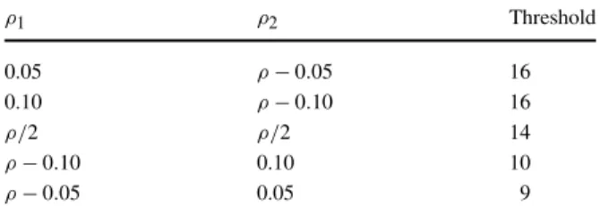
Theorem 2 For Problem1, when there arexicustomers in queueifori=1, . . . , K, it is optimal to select for service the class for whichμii(xi)is maximum.
Proof We use a pairwise interchange argument. Assume that the optimal policy,π, is such that thekth decision chooses classj, the(k+1)th decision chooses classi, and the condition of the theorem is violated. That is,μjj(xj) < μii(xi). We construct an alternative policyπwhere only those two decisions are altered, serving first class ifollowed by classj.
Under both policies, all decisions taken prior to thekth decision and after the (k+1)th decision will incur the same cost. Given the nature of the problem, we can assume with no loss of generality thatk=1 and make use of Lemma1.
So, we can compare the costs of serving first classj followed by classiwith the costs of serving first classifollowed by classj, and the remaining decisions taken according to policyπ.
For policyπ= [i, j, π], we get J
Z(0), π
=C(Z(0))
μi+β + C(Z(0)−ei)
(μi+β)(μj+β)μi+A
Z(0)−ei−ej, π . (18) The termA(Z(0)−ei−ej, π)represents the cost to go after the second service is concluded, and policyπ is used from then on, taking into account that a classi customer was served followed by a classj customer in the first two services.
For policyπ= [j, i, π], we get J
Z(0), π
=C(Z(0))
μj+β + C(Z(0)−ej)
(μj+β)(μi+β)μj+A
Z(0)−ei−ej, π . (19) By the nature of the problem, A(Z(0)−ei −ej, π)=A(Z(0)−ei −ej, π ).
DefiningJ=J (Z(0), π)−J (Z(0), π ), we have J =C(Z(0))
μi+β + C(Z(0)−ei)
(μi+β)(μj+β)μi−C(Z(0))
μj+β − C(Z(0)−ej) (μj+β)(μi+β)μj
= 1
(μi+β)(μj+β) C
Z(0)
(μj−μi)C
Z(0)−ei
μi−C
Z(0)−ej
μj
= 1
(μi+β)(μj+β)
−i(xi)μi+j(xj)μj
. (20)
Given that (μ 1
i+β)(μj+β) >0 andμjj(xj) < μii(xi), it follows thatJ <0, which contradicts the optimality assumption for policyπ.
We can apply the same argument for all consecutive decisions where different classes are served. Therefore, from the optimal policyπwe can construct an alterna- tive policy,π∗, for which costs are never worse that those achieved under policyπ, by enforcing the stated rule whenever policyπ fails to adhere to it, and the result
follows.
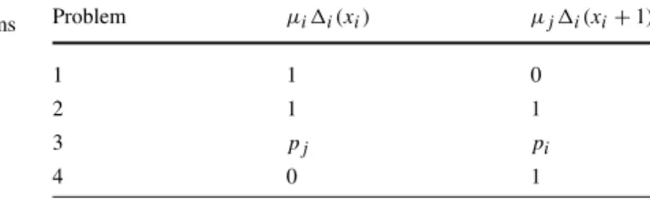
Theorem 3 For Problem2withxicustomers in queueifori=1,2, it is optimal to select for service the classiifμii(xi)+μji(xi+1)is maximum, wherej is the index for the other class.
Proof We use the same proof strategy as for the previous theorem. Assume that pol- icyπis optimal and look for the first decision where the rule is violated. That is, class jis served immediately before classi, with classisatisfying the condition of the the- orem. Next, assume with no loss of generality that to be the first decision, construct a new policy where those two decisions are reversed,π= [i, j, π], and use Lemma1 to obtain
J
Z(0), π
=C(Z(0))
μi+β +C(Z(0)−ei+ej)
(μi+β)(μj+β)μi+A
Z(0), π
, (21) and for policyπ= [j, i, π], we get
J
Z(0), π
=C(Z(0))
μj+β +C(Z(0)−ej+ei)
(μi+β)(μj+β)μj+A
Z(0), π
. (22) Taking the difference of costs for both policies and noting that A(Z(0), π)= A(Z(0), π ), we have
J =C(Z(0))
μi+β −C(Z(0))
μj+β +C(Z(0)−ei+ej)
(μi+β)(μj+β)μi−C(Z(0)−ej+ei) (μi+β)(μj+β)μj
=Ci(xi)+Cj(xj)
μi+β −Ci(xi)+Cj(xj)
μj+β +Ci(xi−ei)+Cj(xj+ej) (μi+β)(μj+β) μi
−Ci(xi+ei)+Cj(xj−ej) (μi+β)(μj+β) μj
= 1
(μi+β)(μj+β)
Ci(xi)(μj+β−μi−β)+Ci(xi−1)μi+Cj(xj+1)μi
+Cj(xj)(μj+β−μi−β)−Ci(xi+1)μj−Cj(xj−1)μj
= 1
(μi+β)(μj+β)
Ci(xi)(μj−μi)+Ci(xi−1)μi+Cj(xj+1)μ1
+Cj(xj)(μj−μi)−Ci(xi+1)μj−Cj(xj−1)μj
= 1
(μi+β)(μj+β)
−i(xi+1)μj−i(xi)μi
+j(xj)μj+j(xj+1)μi
. (23)
Therefore,J≤0, contradicting the optimality assumption for policyπ. The rest of the proof follows the same reasoning presented earlier, and the result follows.
Theorem 4 For Problem 3 with xi customers in queue i for i=1,2, defining pi =λi/2
k=1(λk), it is optimal to select for service the class i if pjμii(xi)+ piμji(xi+1)is maximum, wherej is the index for the other class.
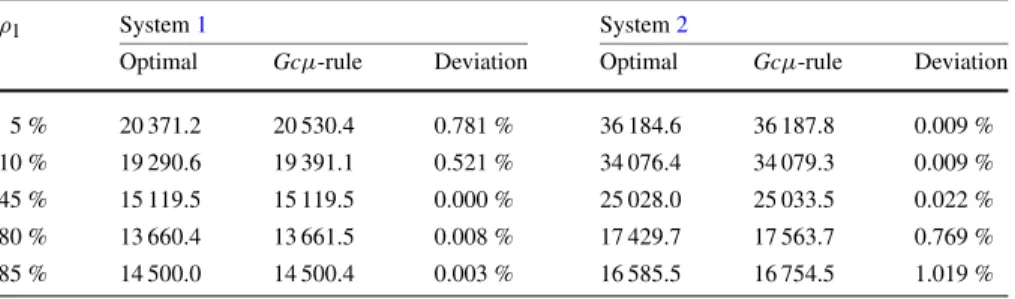
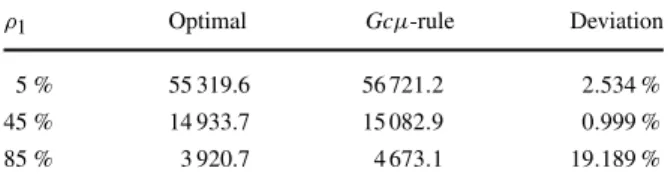
![Table 4 presents V (X, 0) for X = [0 0] achieved with the optimal policy and with Mieghem’s generalized rule, under Gcμ-rule, for the first two systems](https://thumb-eu.123doks.com/thumbv2/123dok_br/19779875.0/23.659.326.584.233.514/table-presents-achieved-optimal-policy-mieghem-generalized-systems.webp)