Introduction
Inter-temporal budget constraints
- Assets
- Expenditure, income and the current account
- The household’ budget constraint
- The government budget constraint
- The economy’ budget constraint
The second term on the right-hand side of (11) is called the government's primary deficit. This equation states the equality between CA and the change in the net international investment position2.
Optimal Consumption
- Preferences
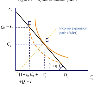
- Euler equation
- Optimal consumption
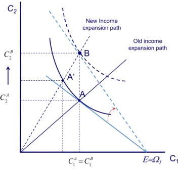
- What happens when the interest rate increase?
Naturally, the question arises as to how current consumption responds to interest rate changes. The intertemporal swap effect is negative because when the interest rate increases, current consumption decreases.
The Ricardian equivalence
Government bonds are not wealth
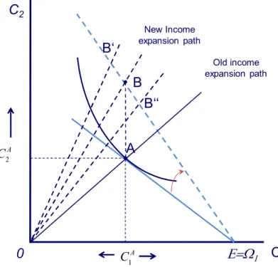
In the case illustrated in Figure 2, these two effects, from A to A' and from A' to B, exactly cancel. Moving away from the notional point B (same as in Figure 2), a leftward shift of the budget constraint means that the household is now poorer.
The Ricardian equivalence
Since government bonds are nothing more than future taxes, issuing government debt only postpones the timing of tax collection. The irrelevance of government debt to consumption decisions is known as the Ricardian equivalence theorem5.
Savings are impacted!
The theorem states that, for any given level of government expenditure, different taxes over time do not affect private wealth or consumption. All in all, the tax cut today only has an impact on the profile of private and government savings without any impact on private consumption and national savings: the fact that households have more disposable income today and less in the future translates into higher private savings today, exactly match the government financing needs brought about by the tax cut.
Macroeconomic equilibrium
Expenditure, Income and Current Account functions
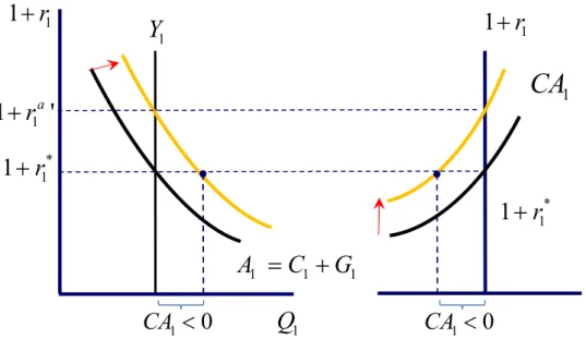
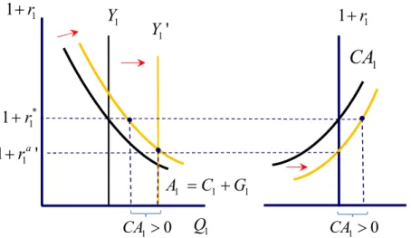
Since a consumer's lifetime wealth 1 is a negative function of the interest rate, national consumption is also a negative function of the interest rate. On the right side of Figure 5, the current account is represented by a positive slope, reflecting the difference between national expenditure and national income.
Open economy
In the same panel, we represent national income (5) with a vertical line (note that in the context of this model output is given, and ro* refers to the last period's interest rate, not the current period's interest rate ). Remember that in this model, the Current Account is also equal to National Savings, because there is no investment: S1 S1P S1G CA1.
Closed economy
If, alternatively, the international interest rate is higher than the autarkic interest rate, it will pay for the country to lend abroad, committing to a current account surplus. Note that the autarkic interest rate in this case is lower than the time preference rate: reflecting the abundance of current consumption relative to future consumption, the price of current consumption must fall enough to force the consumer to choose optimally spending more today than in the future. A question that may arise concerns the meaning of the "autarch" interest rate: after all, if the economy shuts down, which assets trade at that rate.
In fact, the autarky rate will apply to all financial transactions between domestic agents, between private agents and the government, or between heterogeneous private agents. The question is how these quantities are distributed among residential consumers in the first and second periods.
Temporary versus permanent changes in income
- Temporary output expansion
- Anticipated (future) output expansion
- Permanent output expansion
- Change in real wealth
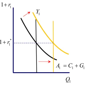
In the left panel, an increase in current output causes the National Income Curve to shift to the right. In the right panel, the curve describing the current account (and national savings) shifts to the right. In this case, household lifetime wealth increases by much more than in the previous two cases (note that a permanent increase in GDP is just the sum of the two changes described above).
In the special case in which r1* , the impact of the permanent change in output on current consumption is one-to-one: an increase in current disposable income is fully matched by an increase in current consumption, implying that the Current Account does not changes to As a consequence, there will be an increase in consumption and an improvement in the Current Account (the savings schedule moves to the right). In the literature, the positive relationship between the terms of trade, savings and the current account is known as the Harberger-Laursen-Metzler effect'12.
As in the two-period case, current consumption responds to the permanent change in income on a one-to-one basis. As in the two-period case, the marginal propensity to consume from current income is less than one. Thus, there will be a current account surplus whenever actual output is higher than the corresponding permanent level.
Government expenditures
Temporary expansion of government consumption
The simplest way to analyze the relationship between demographics and total saving is to assume that society consists of only two groups of individuals: workers and retirees. Returning to the two-period model, assume that all households are identical and that all income is generated in the first period (working life): Q11 and K2 0. Further suppose that the rate of time preference and the interest rate are both equal to zero.
In light of this model, each household will optimally save 0.5 in the first period and save 0.5 in the second period. From the consumer's point of view, a temporary increase in government spending acts as a decrease in actual output: the household will find itself poorer and decide to consume less, through the wealth effect. Due to consumption smoothing, the decline in private consumption in the first period is smaller than the increase in government spending.
Graphically, the effect of an increase in government spending in period 1 is similar to that described in Figure 7: an increase in government spending causes the national expenditure schedule to shift to the right and the CA schedule to the left.
Government consumption and twin deficits
Consider first the case in which an increase in government spending is matched by an increase in current taxes: G1T 10. We conclude that, when the increase in government spending is financed by an equal increase in taxes, Government Savings remain unchanged and private saving falls (the fall in consumption is less than the fall in disposable income). The external imbalance is matched by an imbalance in the private sector: there is no "twin deficit".
Now consider the case in which the increase in government spending is financed with bond issuance. The household buys government bonds amounting to d1G 10 and issues a foreign liability of b1*5, ending up with a net worth of b1 5. In this case, the government deficit translates into an external deficit, generating a pattern of "twin deficits".
Anticipated government expenditures
If the economy is closed, interest rates will fall; if the economy is open, the CA will improve.
Failure of the Ricardian equivalence
The case with borrowing constraints
However, it affects the choice of HTM consumers because they are limited in the amount of current consumption they can buy. There is an effect on private consumption, corresponding to the share of stressed households in the economy. In the case of Ricardian consumers, saving will decrease by the exact amount that must be borrowed from the government.
The only way for the government to use the remaining resources generated by the tax hike is to buy an amount of bonds abroad that matches the decline in consumption of households with restrictions. In summary, in the case of an open economy, a tax increase causes HTM to reduce consumption, leading to a contraction in government spending and an improvement in the current account. This, in turn, requires a capital outflow corresponding to the portion of the government surplus that does not fund Ricardian consumers.
The later must reduce the enough for Ricardian households to expand consumption how enough to borrow the exact amount of the government surplus from the government16.
Inter-generational effects
Distortionary taxation
However, the slope of the intertemporal budget constraint (9c) is affected by the timing of taxation. Since consumption taxes affect the relative price of current consumption compared to future consumption, they appear in the new Euler equation (17c)18. 17 In a closed economy, however, there may be an indirect effect through a change in the interest rate.
18 Note that the distortion only arises because the tax rate is not uniform over time: if 1 and 2 were equal (to finance some positive amount of government spending), there would be no change in the relative prices of current versus future consumption, and thus no distortion in consumption-saving decisions (see exercise on "tax equalization" below). The argument applies only to temporary shifts in government spending: permanent increases in government spending should be met with permanent increases in tax rates. In the case of an open economy, the balance of payments deficit exactly matches the additional private consumption.
In the case of a closed economy, the autarkic interest rate must rise in order for private consumption to decrease (and private savings to increase) enough to finance the fiscal deficit.
Summary
In this economy, current and future GDP are Q1 = 1125 and Q2 = 1350. a) Find the optimal saving in this economy as a function of the interest rate. Suppose further that initially there are no external assets or liabilities and that the world interest rate is r* 5%. a) Find out the value of the country's wealth 1. Assume further that in this economy the interest rate and the time preference are both equal to zero.
In this case, what should the interest rate be in period 1. Imagine a small economy open to international capital flows. Describe the impact of a "sudden stop" in consumption, interest rates, and the current account. Compare with b) using a graph that describes the country's current account as a function of the interest rate.
How much is private consumption, private saving, government saving and domestic interest in period 1? Calculate private consumption and the equilibrium interest rate in this economy, assuming government expenditure equals . Quantify the impact of this policy on private consumption in period 1 and period 2, as well as on interest rates.
Consumption and the interest rate