On the trajectory of a tumbling body Aerospace Engineering

Este trabalho pretende dar um primeiro contributo para a solução deste problema, combinando a teoria da queda livre com o efeito de forças aerodinâmicas não lineares na trajetória de um foguete. Foi desenvolvido um programa capaz de resolver numericamente esta equação, para que a trajetória de um foguete em queda livre possa ser simulada, quando são fornecidas as condições iniciais e dados gerais do foguete.

Nomenclature

Glossary

Introduction

• Motivation
• Safety Procedures During Launch and Flight Termination
• Objectives
• Thesis Outline

The configuration of the standoff systems used by the Challenger space shuttle is shown in Figure 1.1 as an example of payload placement for a solid rocket booster (SRB). In addition to the reliability of the RSS, the placement of the systems on the rocket is also of great importance.

Flight in a Vertical Plane

Theoretical Overview

In the equations 2.2a and 2.2b, the two pairs (x0, z0) and (u0, v0) correspond to the body's initial position and initial velocity components respectively. The use of free-fall coordinates specifies the deviation from the parabolic ballistic trajectory in the presence of uniform gravity alone. The use of free-fall coordinates is a great simplification, as implied by the equation of: 1 - the exact equation of motion which is of first order for the velocityV and flight path angleγ and second order for the angle of attackαso that the system ((equations 2.1a-2.1c)) is of the fourth order; 2 - the approximate equation of motion ((equations 2.5a-2.5c)) which is subsequently shown to lead to a third-order system, by eliminating for the angle of attack.

Solving Equation 2.12 gives the angle of incidence as a function of time α(t), and substituting into Equation 2.6 gives the velocity V(t). The initial conditions for the third-order differential equation are: angle of incidence 2.14a, angular velocity 2.14b, and angular acceleration 2.14c, which follows from the initial velocity (equation 2.6) at time zero. So far, there have been no assumptions about the dependence of the coefficients of drag, lift and pitching moment on the angle of incidence.

Aerodynamic Coefficients Over a Full Circle

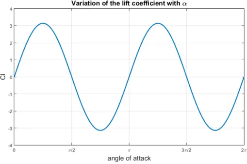
For small angles of attack the cos(α) factor is equal to the 1 and therefore equation 3.2 satisfies the first condition. The variation of the lift coefficient that this theory uses for, for example, a Jowkowski airfoil (CLα = 2π), is the one presented in figure 3.1. The wake coefficient specified in equation 3.7 is only valid for angles of attack between 0 and π2.

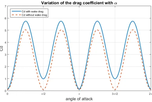
Finally, the drag coefficient will be given by the sum of friction drag, induced drag and wake drag. Putting all the aerodynamic coefficients in the form of equations 3.2, 3.5 and 3.8, it is possible to combine them with the equations of motion (equation 2.5b-2.5c). In accordance with the substitution of equation 3.5 in equation 2.6 and according to the transition from 2.6 to 2.7, using this result in equation 3.9a results:. which is then expanded in several steps.

The first step is to solve the time derivative of the right-hand side of equation 3.11, similar to the transition from 2.7 to 2.8. 3.12). On the right side of equation 3.14 appear two dimensionless parameters that do not depend on aerodynamic coefficients.

Analytic Solutions for Small Angles of attack

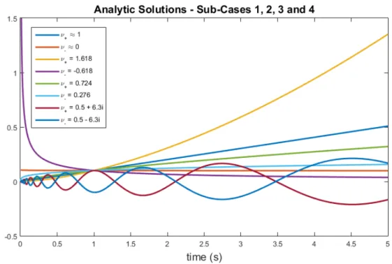
The negative sign in equation 4.6 makes the dimensionless parameter positive (in most cases), since for the rocket to be stable, CMα must be negative. In this case, the roots of equation 4.8 are expanded to any power between 0 and 1 (4.19b), leading to the angle of attack solution from equation 4.10c. The velocity can be obtained by substituting the roots of ν± (equation 4.19b) into the velocity equation (4.12) from the second case.

Similar to the angle of attack solution (equation 4.20c), the flight path angle will have an oscillatory behavior. Solving the limits at time zero and infinity for the angle of attack (Equation 4.20c), velocity (Equation 4.22) and flight path angle (Equation 4.23) leads to the same results for ν+ as in the second case (Equations 4.17a and 4.17b). The first effect is the angle of attack caused by the pitching moment (equation 2.5c).

The second competing effect is a monotonic increase in angle of attack caused by drag (equation 2.5a). In most cases solving the positive root ν+ from equation 4.8 leads to a faster mode (the angle of attack increases faster) than with the negative root ν−.

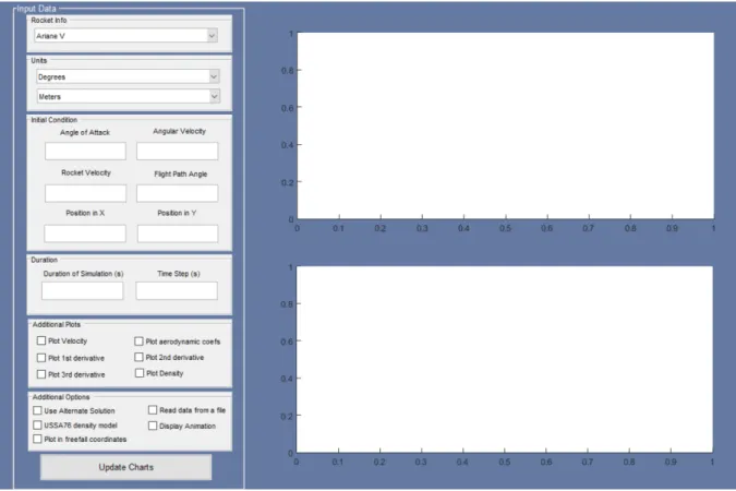
Implementation

• Numerical Model
• Program Overview
• Read initial information
• Integration Process
• Density Model
• Integrator Choice
• Data Treatment
• Program Limitations and Enhancements

Reading values ​​for initial conditions and their units, simulation duration and selected time step. In addition to the initial conditions, the user must also specify the duration of the simulation and the time step to be used. The "plot options" check boxes allow the user to obtain additional plots at the end of the simulation (velocity, angular velocity, etc).

The “Additional Options” checkboxes allow the user to make changes to the default models used during the integration process, or play an animation at the end of the rocket motion simulation. When analyzing the steps for this phase, shown in the flowchart (5.2), most of the steps are solved in the. The final steps of the integration process phase are an update of the initial conditions (replaced by the values ​​obtained by the current integration) and a check to see if the entire phase needs to be repeated for another rocket (occurs only if a text message A file similar to the one shown in Appendix A is used).

All the data calculated during the integration process phase is stored in a solution array. This happens because of the indeterminacy in the angle of attack differential equation mentioned before.

Simulation of tumbling trajectories for a variety of debris

Base Configuration

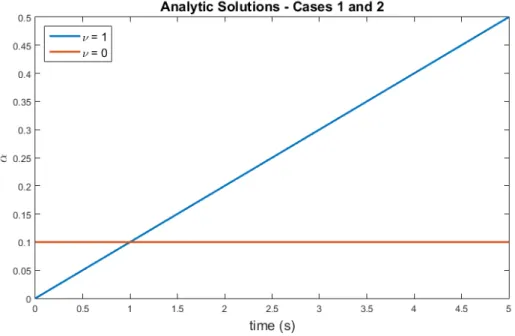
Figures 6.1 and 6.2 respectively depict the trajectory for the 4 possible cases (combination of the 2 configurations and 2 .. α-solutions) and the variations of the angle of attack and the flight path angle versus time. Using the first solution leads to the trajectory that covers the longest distance of the four cases, while using the second solution leads to the shortest distance. In figure 6.2 it can also be seen that the flight path angle remains constant throughout the simulation regardless of the base configuration chosen and the solution chosen for.

Figures 6.3 and 6.4 show the variation of the first and second derivatives of the angle of incidence over time. The second difference can be seen in both the first and second derivatives of the angle of incidence and is a decrease in the amplitude of oscillations. Continuing the analysis, Figures 6.5 and 6.6 show the variation over time of the third derivative of the angle of attack and the derivative of the flight path angle, respectively.

The third derivative of the angle of attack, like all other lower order derivatives of the angle of attack, always has a periodic behavior. The last two parameters subjected to this analysis are air density and rocket velocity shown in Figures 6.7 and 6.8 respectively.

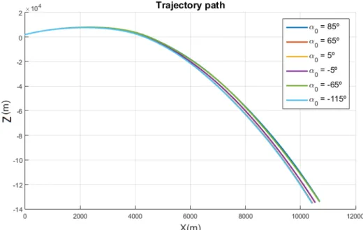
Sensitivity Analysis - Initial Conditions Testing

• Angle of attack
• Angular Velocity
• Velocity
• Flight path angle
• Coordinates x and z

Regarding the effect of the angular velocity on the regime adopted by the rocket, it is clear that a high/low enough initial angular velocity is sufficient to change the initial state of the base configuration (0o/s in the first configuration has an oscillating state and 8o/s in the second configuration leads to a full revolution mode). Analysis of Figures 6.10 and 6.11 leads to different conclusions regarding the effect of angular velocity on the trajectory of the rocket. On the other hand, when the body is in an oscillating state, the initial angular velocity does not have a significant influence on the trajectory of the body.

The angle of the flight path has no influence on the amplitude and period of oscillations or rotations of the angle of attack and all its derivatives, as shown in table 6.5. It is constant throughout the simulation and only changes the trajectory of the rocket, as shown in Figure 6.13. If the constant density model had been assumed instead of the USSA76 model, the same would apply toz0.

Increasing the initial altitude of the missile not only changes the maximum altitude reached by the missile, but also reduces the maximum range of the missile as seen in Figure 6.15. The range decreases because although the initial velocity of all cases is the same, the final velocity of the body is not as can be seen in figure 6.16.

Sensitivity Analysis - Rocket Data Testing

• Mass
• Length
• Radius
• Distance from C.P to C.M
• Aerodynamic Parameters

The only effect of changing the racquet length is changing the maximum and minimum of the pitching torque coefficient over time. The trajectory of the rocket is affected by the radius of the rocket and has contrasting results depending on the initial configuration. The new equilibrium position can be explained by the configuration of the rocket for positive values ​​of a being an unstable configuration from the start.

An increase/decrease of this parameter instantly increases/decreases the value of the resistance coefficient. The most significant change caused by varying the frictional resistance occurs in the trajectory of the rocket, as seen in Figure 6.25. By analyzing the trajectory of the rocket for the different values ​​of frictional resistance, the immediate conclusion is that for lower values ​​of CD0 the rocket reaches a higher horizontal distance.

The angle of attack amplitudes is not affected by the changes to the frictional resistance, but the period of the oscillations increases with the frictional resistance. This result is also expected because for lower resistance values ​​there is less resistance in the path of the rocket and consequently the rocket completes its oscillations faster.

Conclusions

Future Work

This could include adding more rocket families to the menu and finding more accurate ways to measure values ​​like the rocket inertia. Redo the equations of motion of the rocket to include 3D motion instead of 2D and implement those equations in the program. Make a video recording a free-falling rocket (with known characteristics) and compare the resulting trajectory with the program prediction.

Consider the Earth's rotation and the Coriolis effect when calculating the debris path.

Bibliography

27] Report to the President of the Presidential Commission on the Space Shuttle Challenger Accident, Part III, Appendix O: NASA Search, Recovery and Reconstruction Task Force Team Report, June 1986. On the Effect of Nonlinear Aerodynamic Forces on tumbling trajectory of a debris, manuscript, 2017. Preliminary definition of an aerodynamic configuration for a reusable booster stage within tight geometric constraints. Proceedings of the Fifth European Symposium on Aerothermodynamics for Space Vehicles, pages 21–27, February 2005.

Appendix A

Text File Format

Appendix B

ODE23s method