These qualitative aspects of the phase diagram corresponding to the disordered Bose-Hubbard model were first investigated in [22]. In the presence of disorder, translational invariance is broken due to local imperfections of the random network.
Outline of the thesis
For this purpose, we derive the spectral function that follows from the partial summation result of the Green's function. First, we derive the superfluid phase boundary from the partial summation result of the Green's function.
Theoretical background
Cold atoms in random optical lattices
AC-Stark effect
This result points to the fact that the polarization of the atom oscillates at the same frequency as the external electric field and thus the energy shift acts as an effective trapping potential for the atom. Additionally, we introduced ε, which is a unit vector that determines the direction of the electric field.

Optical lattices
By controlling the interference angle between the laser fronts, the grating spacing can be changed to produce different geometries such as triangular [62] and Kagomè [63]. To understand how to investigate the effects of disorder in such structures, we review some of the most common experiments.

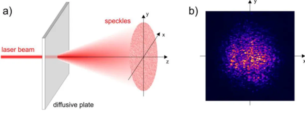
Speckle laser disorder
The size of the randomly sized light intensity grains that characterizes the speckle pattern can be inferred from the width of the intensity autocorrelation function. This is the correlation between the intensities of the random pattern at different spatial points.
Bose-Hubbard model
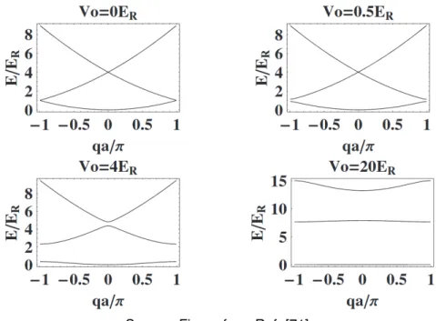
- Single-particle band structure
- Bose-Hubbard Hamiltonian
- Hamiltonian parameters
- Ground states of the Bose-Hubbard model
Competition between the parameters of the Bose-Hubbard Ovega Hamiltonian leads to different ground states. A schematic drawing of the different states of a double well can be seen in fig.
Detection
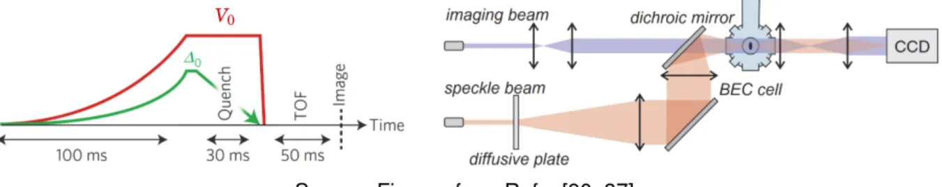
- Time-of-flight imaging
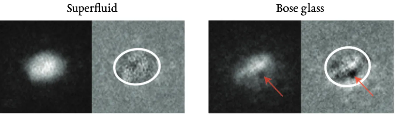
- Experimental characteristics of the ground states
We now discuss the characteristics of the phase transitions between the various Bose-Hubbard Hamiltonian ground states. In the case of the superfluid phase, the density profile shows nothing but a continuous background due to the macroscopic phase.
Superfluid to insulator phase transition
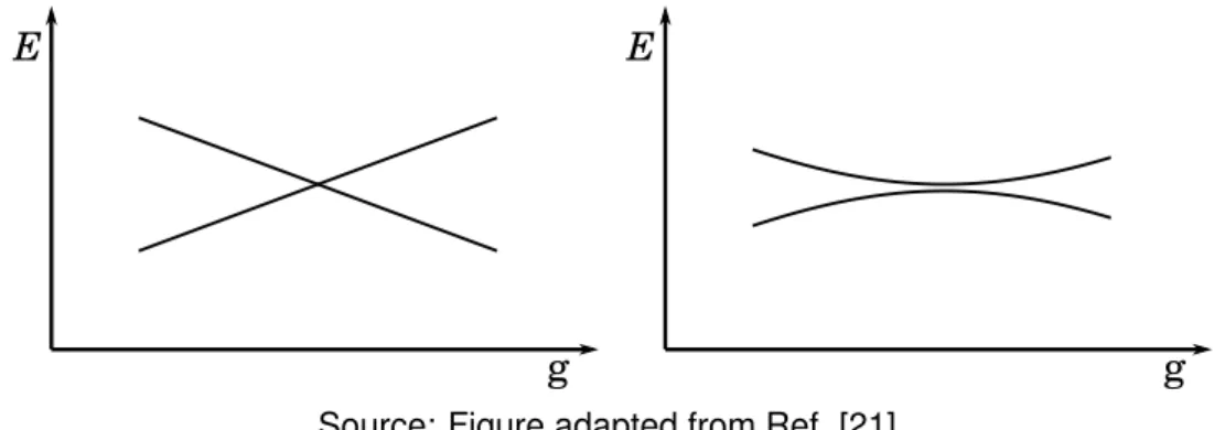
- Quantum phase transitions
- Landau Theory
- Zero-temperature phase diagram for the clean system
- Zero-temperature phase diagram for the disordered system
A qualitative picture of the phase diagram in the disordered case can be observed in Fig. In the situation where all such regions are on the same side of the phase transition, i.e. in the case of the disordered Bose-Hubbard model, it is characterized by the emergence of the Bose-glass phase.
Single-particle Green’s functions
Linear response
To investigate the response of the macroscopic system to the external disturbance, one must solve the above equation. Equation (3.5) is a solution of (3.2) in the absence of the perturbation Hˆ1 provided that the unperturbed Hamiltonian oscillates with the number operator Nˆ, i.e. The above equation defines the so-called Green's function, which characterizes the system's linear response to an external disturbance.

Källén-Lehmann representation
Using Heaviside's step functions, the time-ordered Green's function can be written as 3.30). Note that the analytic continuation also causes the poles of the Green's function to shift. An essential detail about such a general result is that it implies that the Green's function in Fourier space is a meromorphic function of frequencies.
Spectral function
An important feature of the spectral function is that it is possible to recover the full Green's function by integration over the frequency domain. The spectral function then becomes a central feature, as it can be used to obtain the Källén-Lehmann representation of important Green's functions. An important property of the spectral function can be proved by considering the integral of the inverse Fourier transform.
Imaginary time and Matsubara formalism
However, one must ensure that this analytic continuation leads to a unique representation such that the asymptotic behavior of the Green's function is large. We have derived key aspects of the green functions and spectral functions relevant to our analysis. Therefore, next we will focus on the general properties of Green's function and spectral functions in disordered systems.
General properties in disordered systems
Therefore, in the following, we will focus on the general properties of the Green's function and the spectral function in disordered systems. the representation of the disordered potential in reciprocal space becomes X. 3.65). Thus, we can expect that instead of the delta distribution in k-space shown in (3.32), the Källén-Lehmann representation of the Green's function in the disordered case will involve a superposition of states with different momentums. However, since the disordered mean in (3.61) is supposed to converge and therefore commutes with the trace of definition (3.19), the mean Green's function becomes statistically homogeneous and the translational symmetry is restored.
Physical interpretation: elementary excitations
Therefore, the key information about the excitations can be obtained from the singularities of the Green's function in frequency space. Such a quantity can be defined from the imaginary part of the Green's function in space. We demonstrate the concepts that connect the Green's functions to the propagation of the excitations in Chapter 5.
Bose-Hubbard model in the limit of strong interactions
Therefore, in the limit of strong interactions, the entire Matsubara Green's function can be written as As discussed earlier, the simple poles of the Green's function in the pure case are mapped to the peaks of the Dirac delta distribution of the imaginary part. This can be understood if we remember that in the pure excitation case the real eigenstates are the Hamiltonian.
Measurements in disordered systems
- Bragg spectroscopy
- Radio-frequency transfer
The dynamical structure factor measures fluctuations in the density-density correlations of the many-body system. In the presence of disorder, one must consider the average of the transition rate over many realizations of the random potential. 3.5(d) and (e) that the spectral function has a peak indicating the excitation energies of the disordered potential.
Perturbation Theory
Hopping expansion
Since we want to study the system near the phase transition, we introduce a source term to the action. Here we restrict the calculation to the two-point Green's function which can be obtained from [141]. To properly calculate the hope corrections to the Green's function, we must take into account the cumulant expansion of the free energy.
Partial summation
We emphasize that this result is equivalent to the partial summation of simple chain contributions to the Green's function obtained for the pure case in [99] and for the disordered case in [139, 140]. In an actual disordered system, the reciprocal space representation of the Green's function must have non-diagonal elements that connect states with different wave vectors. In the next section, we show how information about the energy spectrum for single-particle excitations can be obtained from such a quantity.
Poincaré-Lindstedt method
The hopping corrections of the local density of states (4.23) are multiplied by the derivatives of the disorder distribution. By analogy with the Poincaré-Lindstedt method, we suggest using the following transformations. The renormalization of the disorder distribution arguments in the local density of states can therefore be interpreted as the Poincaré-Lindstedt method in frequency space.
Results
Excitations of the disordered Bose-Hubbard model
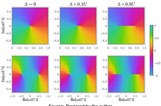
Spectral function
- Clean case
- Disordered case
The spectral function is defined as the imaginary part of the retarded Green's function (3.37). Therefore, the peaks of the spectral function correspond to the frequencies that make up the first term of v. Such information is mapped to the finite width of the spectral function in this range.
Uniform disorder distribution
- Mott lobe n 0 = 0
- Mott lobe n 0 = 1
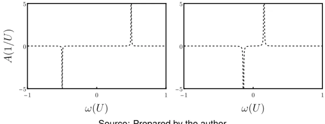
- Green’s function in space time
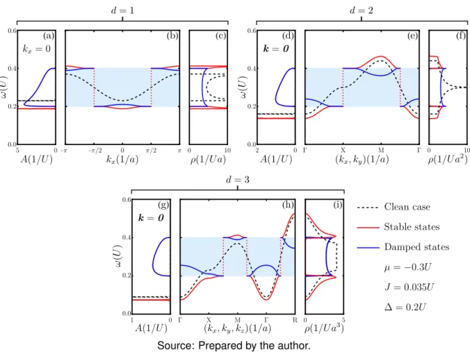
We note that the strong peak of the steady states in the disordered case (red) is shifted towards lower energies compared to the steady states of the pure case (dashed black). 5.5(a), the effects of disorder are clearly demonstrated by the increase in the effective mass of the steady states. Moreover, we conclude that the amplitude of propagation of the full Green's function in Fig.
Summary of results
Phase diagram at finite temperatures
- Superfluid phase boundary
- Local density of states
- Mott insulator to Bose glass phase boundary
- Comparison with numerical results
- Summary of results
This expression for the phase boundary is a generalization of the results obtained in the case where disorder is present. Note that, in this approximation, hopping contributions appear in the argument of the disorder distribution. This result corresponds to the analytical expression of the phase boundary between Mott insulator and Bose glass.
Preliminary calculations
Superfluid elementary excitations
- Effective-action approach
- Excitation spectra in the Mott-insulator phase
- Excitation spectra in the superfluid phase
- Bose-glass spectra
Furthermore, the effective function evaluated at the equilibrium value of the order parameter is equal to the free energy. As a result of the Legendre transformation, the effective action can be expressed as an expansion in the field of the order parameter given by . 7.14). To obtain analytical information about the excitation spectrum, we can study the fluctuations of the effective operation around the equilibrium value of the order parameter.
Free lattice bosons with weak disorder
Disorder expansion
Completing the square in the argument of the exponential function in the numerator of (8.1), we get. However, in the present case we can see that the real part of the self-energy shifts the distribution ratio of the excitations. Considering that the peaks of the spectral function are still close to the undisturbed dispersion,ω0(k)= −µ−J(k), we can estimate such a lifetime as.
Single-site approximation
The following is a description of how to obtain the explicit form of one's own energy using the one-point approximation. In the previous analysis performed in Chapter 5, the logarithmic branch cut represented the mathematical signature of damped-localized excitations. Thus, the presence of such a branch cut in this calculation can be interpreted as a sign of the appearance of these damped-localized excitations.
Final remarks
Summary and conclusions
Svistunov, "Phase diagram and thermodynamics of the three-dimensional Bose-Hubbard model," Physical Review B, vol. Svistunov, "Phase diagram of the corresponding two-dimensional disordered Bose-Hubbard model," Physical Review Letters, vol. Gooding, "Application of a multisite mean-field theory to the disordered Bose-Hubbard model," Physical Review A, vol.
Functional-integral formalism
Lattice occupation number representation and Fock space
Given that such Hamiltonians are conveniently expressed in terms of the creation and annihilation operators, the idea would be to look for the eigenstates of such operators.
Coherent states
We now have a normalized basis of the Fock space in terms of the coherent states. To derive the overcompleteness relation, we define the following operator Iˆ=. where the integration runs over the entire complex plane. A general array element of this operator can be written as. using the polar coordinatesψi=reiφ andψ∗i =re−iφ the integration becomes Zdψ∗idψi. A.14).
Imaginary-time path integral and the partition func- tion
Therefore, the partition function can be considered as the sum over the diagonal matrix elements of the imaginary-time evolution operator Uˆ(τ,τ0)=e−(τ0−τ). The integration of the second term, corresponding to the damped states, is more involved. 2−4J(k)2π2l(1+l)+2iπ∆J(k)(1+2l)¤2, (B.6) where the first term stands for the residue of the singular pole in the upper half of the complex plane on the denominator of the right side of (B.5), while the second term consists of the sum of infinitely many residues in the upper half of the complex plane that comes from the hyperbolic secant function in the numerator.