The model's calibration reflects a typical OECD economy and takes into account a breakdown of households by income quintiles. It assesses the effects of a tax reform that eliminates the progressivity of the tax on labor income while maintaining or increasing the progressivity of the tax on capital income.
Introduction
From the point of view of the prosperity index, public investment is the best instrument to consolidate public debt. 9 They believe that the best change in the fiscal mix to increase output in the long run (by about 2%) is to reduce government consumption, coupled with a reduction in the capital income tax rate.
Model Specification
Households
1 + 𝜏𝑡𝑐)𝐶𝑡𝑁𝑅 = (1 − 𝜏𝑡𝐿𝑁𝑅)𝑤𝑡𝑁𝑅𝑍𝑡𝑁𝑍𝑡𝐻𝑡𝑁+ 𝑡𝑟 (1.7) where the left side indicates that the only use of income is for consumption (𝐶𝑡𝑁𝑅) after deducting its ad valorem tax, with a rate of 𝜏𝑡𝑐. The right side indicates that the sources of income are:. i) the product of the wage (𝑤𝑡𝑁𝑅), the number of hours worked (𝐻𝑡𝑁𝑅) and the exogenous productivity of labor (𝑍𝑡), net of the ad valorem labor income tax, with rate 𝜏𝑡𝐿𝑅; and (ii) the share 𝜔𝑁𝑅 of average government transfers to households (𝐺𝑡𝑡𝑟). 𝐿𝑅𝑡 + 𝐻𝑡𝑅 = 1, and 𝐿𝑁𝑅𝑡 + 𝐻𝑡𝑁𝑅 = 1 (1.8) The solution of the planning problem of each of the two household types therefore takes the fiscal policy parameters as,𝑡se, the government 𝑅, 𝑤𝑡𝑁𝑅, 𝑟𝑡𝑡𝑅𝑅, as given and, from the initial values of the variables, yield trajectories {𝐶𝑡𝑅, 𝐿𝑅𝑡, 𝑡, 𝑐, 𝑐 𝐷𝑡𝑅, 𝐾𝑡+1𝑅 , 𝐵𝑡+1𝑅 }𝑡=0∞ and {𝐶𝑡𝑁𝑅, 𝐿𝑡𝑡𝑐𝑡𝑐 }𝑡=0∞.
Firms
𝐾𝑡+1𝑅 = (1 − 𝛿𝑝)𝐾𝑡𝑅+ 𝐼𝑡𝑅 (1.5) 𝐵𝑡+1𝑅 = 𝐵𝑡𝑅+ 𝐷𝑡𝑅 (1.6) Non-Ricardian households do not own shares in companies or physical capital, and therefore do not receive dividends or capital income , and neither lend nor borrow, so their budget constraint is: The equilibrium of factor markets requires that aggregate demand, derived from equations (1.10) and (1.11), be consistent with supply.
Government
24 This very simplified formulation of economic openness is sufficient to capture the crucial fact that foreign savings inflows have historically been an important source of funds for financing Brazil's budget deficit, and proves to be very useful to calibrate the model. in line with recently observed government expenditure ratios.
Equilibrium
The latter are rates of the ad valorem tax on consumption, on labor and on capital income (𝜏𝑡𝑐, 𝜏𝑡𝐿𝑁𝑅, 𝜏𝑡𝐿𝑅, 𝜏𝑡𝑘) and average household government consumption, 𝑔 𝑡𝑖, 𝑔𝑡𝑡𝑟). The numerical solution of the system yields dynamic equilibrium perfect prediction trajectories of the variables.
Calibration of the Model for the Brazilian Economy
According to Papageorgiou (2012), the growth rate of GDP per per capita in the United States (2% per year) used for the labor force growth rate that increased technical progress 𝛾𝑧.28 The initial level of the technical progress parameter (𝑍0) was set to one. The depreciation rate for total physical capital was set at 3.5% per year, which is the value that Gomes et al. 2003) by applying the permanent calculation method to the National Accounts' investment series.

Fiscal Policy Simulations
Long-run Effects of Fiscal Mix Changes
- Best policies to increase steady-state (SS) output
- Best policies to increase steady-state (SS) consumption
- Best policies to increase SS welfare
- Effects on labor, capital, wages and returns to capital
The difference in the result of the models is most likely due to the previously indicated difference in the calibration. Some of the effects in the variables shown in the simulations can be traced back to the comparisons.
Dynamic debt consolidation policies
- Effects on output
- Effects on consumption
- Effects on labor
- Effects on private investment and capital stock
- Effects on public capital stock
- Effects on public debt and deficit
- Welfare effects
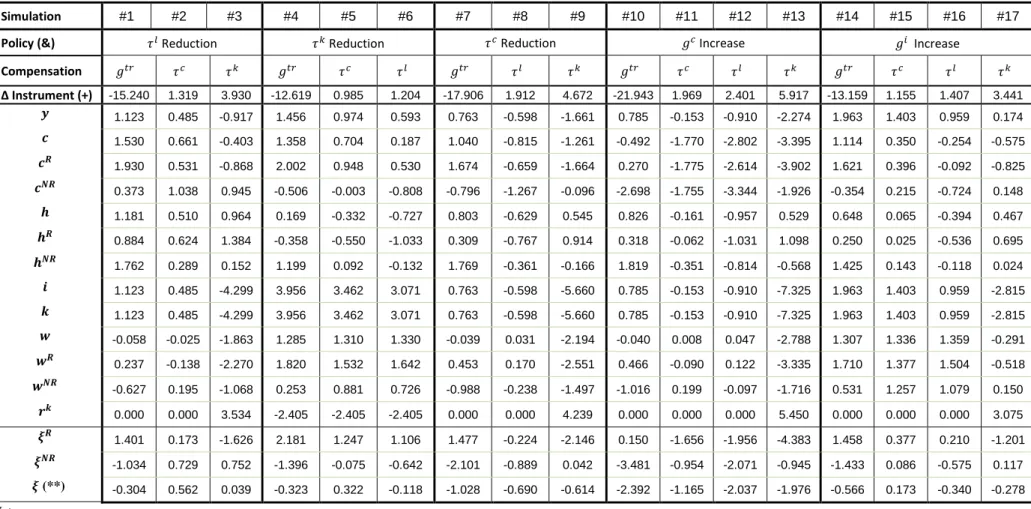
This is due to the effect of a smaller tax rate on capital income in private investment (𝑖) and in the build-up of private capital stock (𝑘), which increases by 2.7% in the long run. However, the ranking of the policies based on the long-term effect is the same in the two versions of the model. The long-term changes in the primary deficit-to-output ratio (𝑑 𝑦⁄ ) in Table 1.3 range between 0.35 p.p.

Concluding Remarks
The effect of these last two policy measures on the consumption of the two types of households is asymmetric. On the other hand, the increase in consumption of non-Ricardian households of the second policy amounts to 74%. From that perspective, the best policy is neither of the previous paragraphs, but it is.
Introduction
They also describe the transition dynamics of the economy to achieve this long-term equilibrium. This is an example of the recent debate in the US and several other countries about raising the marginal tax rate for the highest income households. 63 Summers (1982) and King and Rebelo (1990), among others, point to the importance of EIS for the effect of fiscal policy on long-term equilibrium in representative agent models.
Model Specification
Production technology
𝐾𝑗 is the private capital stock, 𝐿𝑗 is the input of labor services into production, 𝐾 is the average total capital stock in the economy, and A is the scale parameter. This production function is consistent with endogenous growth because it exhibits constant returns to scale with respect to 𝐿𝑗 and 𝐾𝑗, as well as to 𝐾𝑗 and 𝐾. The term 𝐿𝑗𝐾 is the labor input in efficiency units.66 Since firms are assumed to be identical, 𝐾𝑗 = 𝐾 and 𝐿𝑗 = 𝐿, and the aggregate production function is a linear function of the average total capital stock:. When 𝑙 denotes the average leisure in the entire economy, so that 𝐿 = 1 − 𝑙, the wage rate (𝑤) and the return to capital (𝑟) must satisfy the following equations.
Households
The first term on the right-hand side is income from capital, and the second term is income from "raw" labor, i.e. For each household, the tax rate of each factor depends on the amount of goods supplied relative to the amount in the average household, and the corresponding tax rates (𝜏𝐿𝑖) and (𝜏𝑘𝑖) are given by . The average and marginal tax rates are a weighted average of the individual rates, with their relative capital gains as weights, as follows.
Government
The rules for combining income, capital and free time and calculating aggregate labor and capital markets are as follows: 69.
Equilibrium
We can now show that the progressive tax structure can lead to a unique non-degenerate distribution where wealthier households with a higher EIS end up owning a larger share of wealth. Assume that the tax rate on capital is progressive 𝜙𝑘 > 0 and that the individual from group 1 has a higher EIS compared to the individual from group 2, i.e. that the dynamic reactions of the economy to the change in the tax schedule are given by the dynamic system consisting of The 𝑁 − 1 accumulation equations (2.19), the 𝑁 − 1 relative (gross) income equations of (2.20), the 𝑁 equations (2.23) and the aggregations defined in (2.11).
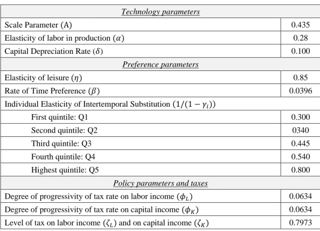
Calibration for a representative OECD country
The EIS distinction between income classes is of crucial importance in determining their heterogeneous behavior of households in model simulations, and its calibration is supported by several studies in the literature. 76 In 2019, the average hours worked per week in the US by persons who usually work full time was 42.5, according to the US to calibrate the EIS in this chapter's model, which has five types of households corresponding to quintiles of the income distribution incomes. , its value for each class is determined according to the evidence in the previous paragraph, as follows.
Benchmark equilibrium and policy simulations
Scenario A - Flat taxes on labor income
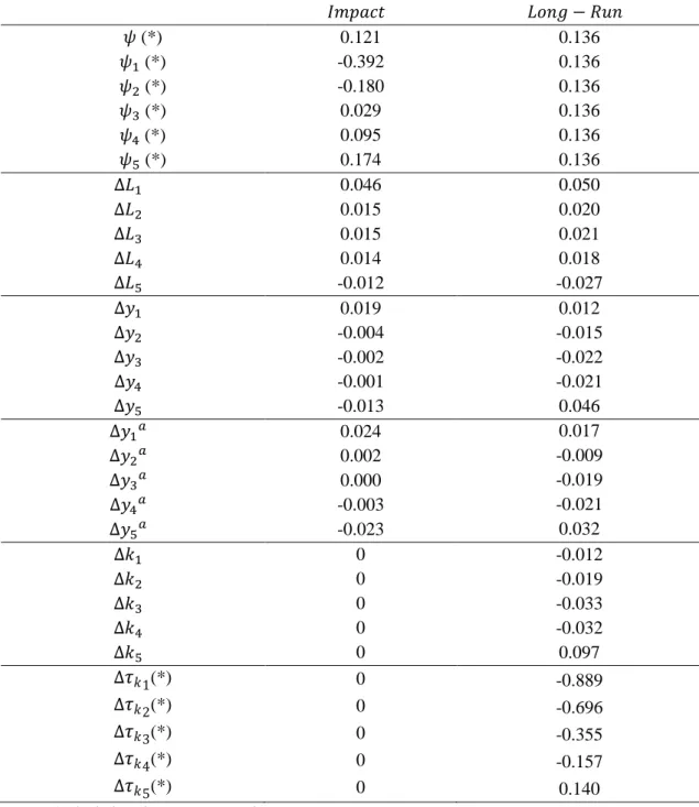
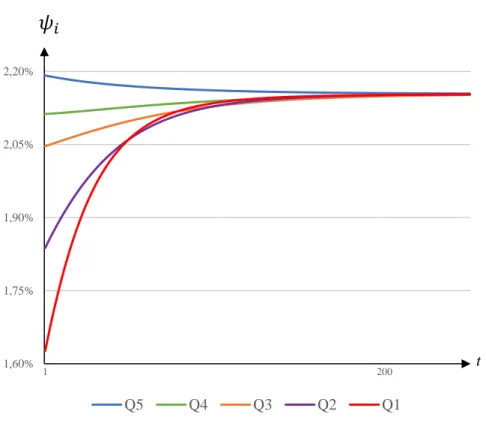
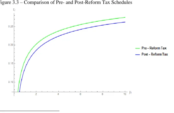
81 The pre-reform tax rate on labor income was a function of the agent's labor supply. 5 presents the quintiles of the income distribution. a) the variables Δyia are the proportional change in the disposable income of the ith quintile. In contrast, for the bottom quintiles, the effect of the reduction in consumption taxes is strong, resulting in a reduction in the rate of asset accumulation.
Scenario B - Flat taxes on labor income and more progressive capital taxation
Summarizing the effects of removing progressivity from labor taxation, as simulated in this scenario, we see a modest trade-off between growth and inequality in the long run. The policy's effects on total tax revenues are surprisingly small, falling by only 0.1 percentage points. The net effect is an immediate, short-term decline in total (and average) capital, leading to a decline in the growth rate of the economy's accumulation (𝜓=−0.133).

Concluding Remarks
In summary, the fiscal policy of scenario B, which complements the removal of the progressivity of labor income taxation with the increase of the progressivity of capital income taxation, avoids the troublesome results of scenario A and provides an equilibrium that shows the expected negative effects on the growth of policies designed to reduce inequality. In summary, the results show that the degree of progressivity of the tax rate on capital income plays a crucial role in determining the impact of structural changes on growth and inequality. The dramatic drop in the GINI coefficients in scenario B reveals that increasing the progressivity of capital income taxation is effective in tackling inequality, but at the cost of reducing the overall growth rate of the economy, both in the short and long term.
Introduction
The model proposed here has several characteristics of the model from the previous chapter. The first extension, detailed in the next section, leads to a more realistic reproduction in the model of the observed US tax code. In the numerical simulations, we also use a version of the model that takes into account both sources of heterogeneity: differences in the elasticity of intertemporal substitution and in the degree of time preference.
Model Specification
Also, if there is no progressivity (𝜙 = 0), the schedule is flat and the tax rate is independent of the agent's relative income (𝜏𝑖 ≡ 𝜌 − 𝜁). In the literature there are alternative formulations of the tax plan, and the main one is Li and Sarte (2004), which however has some drawbacks. 94 None of the other papers adopting the formulation in Guo and Lansing (1998), cited in the text, consider the extension proposed here.
Equilibrium
However, with progressivity, there is an interaction between the tax scheme and income distribution, and equilibrium aggregates and their distribution among households become jointly determined. The next section describes the steady state of the dynamic system, and the next one uses the numerical solution of a calibrated version of the model to discuss the policy implications of tax reform. In the general case of elastic labor supply, the effect is not so obvious because of the possibility of jumps in 𝐿.
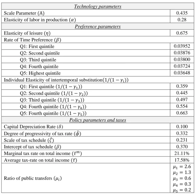
Calibration for the USA before and after the TCJA 2017
Calibration of the tax function
The tax code specifies that, after taking the standard deduction, the application of the marginal tax rate to each successive part of income, up to the tax bracket of the total income of the individual. The estimation of the parameters before and after the TCJA follows a procedure analogous to the one described in Carneiro et al. The range of the parameters 𝜙̂𝑖 and 𝜁̂𝑖 form the upper and lower bounds to estimate these average fiscal parameters.

Calibration of the other parameters
- Technology Parameters
- Preference Parameters
Quite similar to Carneiro et al. 2022), the volume parameter of the production function was calculated as A = 0.435 to obtain an equilibrium growth rate of the economy of about 2.5% per year, which is roughly the same as the growth rate observed in the US economy recently. Evidence in the literature on EIS variations for different income classes is sparse. 108 A more significant change is in the EIS of the richest quintile and is a result of the adopted tax parameters.
Benchmark equilibrium and policy simulations
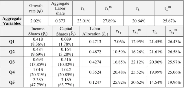
Benchmark equilibrium
It is also compared with the CBO observed values of income before taxes and transfers in 2017 of 3.8% and 54% respectively.111 The share of the capital of the highest income quintile in total assets is 𝑘5⁄ =68 .5%, while the share of the lowest incomes is actually negative. One of the few studies that provides estimates of the share of quintiles in household wealth is Davies et al. 𝑁 ∑𝑁𝑖=1𝑦𝑖 (3.21) It yields a value of 0.434 for the benchmark economy, which is slightly larger than indicated by the latest available data for the US according to the World Bank (0.41) and the OECD. The GINI coefficient for wealth is analogous to that for income, and its value is 0.67, which is similar to the actual values.

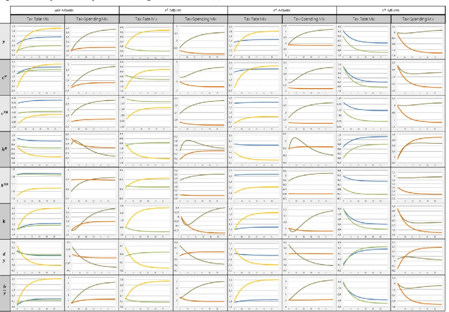
Effects of TCJA 2017 in an economy with one source of heterogeneity
The simulations here and in the next section assume that the tax change of the reform is permanent and that the economy will eventually converge to a new steady state at an endogenously determined rate. 115 A discrete-time version of the model programmed with the General Algebraic Modeling System (GAMS) software described in GAMS (2013). Fiscal reform increases wealth inequality more than income inequality, as the ratio between the GINI coefficient for income and wealth decreases slightly in the long run.
Effects of TCJA 2017 in an economy with two sources of heterogeneity
Their comparison with respectively Table 3.7 and Figure 3.4 shows the differences in the effect of the policy in the two versions of the model. The simulated effects of the TCJA 2017 in the extended model produce the same long-term effect on economic growth, while affecting the distribution of income less than in the original model. A Survey of the Role of Fiscal Policy in Addressing Income Inequality, Poverty Reduction and Inclusive Growth.