Esse índice revela o perfil térmico da comunidade, que é ponderado pela quantidade de espécies que a compõem (DEVICTOR et al., 2008). O clima também pode interagir com outras ameaças à biodiversidade, como espécies invasoras (HELLMAN et al., 2008; RAHEL; OLDEN, 2008). Os primeiros efeitos das mudanças climáticas foram observados nas comunidades de peixes estuarinos (MCLEAN et al., 2019; KIMBALL et al., 2020).
Introduction
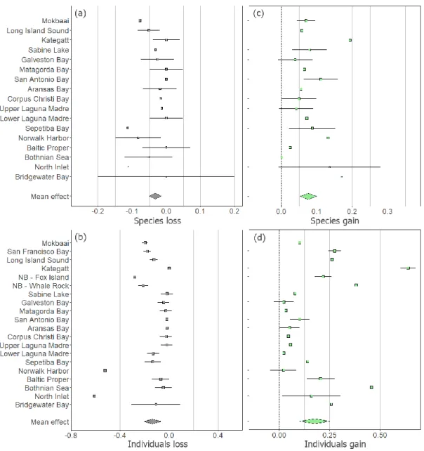
These processes result from the decomposition of the Community Temperature Index (CTI), which measures the abundance-weighted average thermal affinity of any given community (DEVICTOR et al., 2008). Conversely, communities where loss prevails (i.e. deborealization) are more prone to population crashes and local extinctions in the near future (MCLEAN et al., 2021). New communities emerge from shifts in species occurrence and abundance over time (DORNELAS et al., 2019), and both of these components of biodiversity depend on temperature.
Materials and methods
- Search strategy
- Article screening and eligibility
- Data extraction and transformation
- Temporal change in fish assemblages
- Meta-analysis
- Community Temperature Index (CTI) and process strength
TBI values were calculated from the occurrence matrix and species abundance (i.e., density) using the TBI.R function (LEGENDRE, 2015) in the adespatial package (DRAY et al., 2020) for R software (R CORE TEAM, 2020) . The mean thermal affinity of fish assemblages was calculated for the early and late periods and the entire time series of each estuary using the Community Temperature Index (CTI; MCLEAN et al., 2021). Euclidean dissimilarity distance (1000 permutations) was used for PERMANOVA tests, which were performed using the adonis2 function in the vegan package (OKSANEN et al., 2020) for R software (R CORE TEAM, 2020).
Results
- Review descriptive statistics
- Temporal change in fish community
- Meta-analysis
- Community Temperature Index and process strength
The letters indicate the estuarine systems assessed in this review: A – Bothnian Sea; B – true Baltic; C – Kattegat; D – Bridgewater Bay; E – Mokbaai; F – Sepetiba Bay; G – northern inlet; H – Port of Norwalk; I – Long Island Sound; J to Q - bays on the Texas coast; R - San Francisco Bay; S – Narragansett Bay (Fox Island); T – Narragansett Bay (Whale Rock). Note that data from Narragansett Bay (i.e., NB–Fox Island and NB–Whale Rock) and São Francisco Bay are not shown in meta-analyses of species gain and loss, as these studies only reported the occurrence of the most common fish species (FO%>95% ). Bridgewater Bay -0.192 Borealization Residents Sepetiba Bay -0.153 Detropicalization Residents Matagorda Bay -0.01 Borealization Residents Baltic Proper -0.004 Borealization Residents Sabine Lake 0.004 Tropicalization Residents Upper Laguna Madre 0.013 Tropicalization Residents Galveston Bay 0.014 Deborealization Residents Both Nian Sea 0.019 Tropicalization Residents Lower Laguna Madre 0.036 Deborealization Residents of Aransas Bay 0.057 Tropicalization Residents San Antonio Bay 0.068 Tropicalization Residents Corpus Christi 0.091 Tropicalization Residents.

Discussion
Similar results were reported by MCLEAN et al. 2021), which revealed wider thermal ranges for cold-affinity species that promote borealization. Climate change on a global scale affects local factors and shapes the response of individuals to new environmental conditions (GERVAIS et al., . 2021; DUBOIS et al., 2022). However, resident species inhabiting these systems often show phenotypic variation to cope with the heterogeneity of environmental conditions (GERVAIS et al., 2021).
Materials and methods
- Animal collection and husbandry
- Reciprocal-cross experiment
- Silversides’ vulnerability to temperatures predicted for 2100
- Temperature’s isolated effect on CTMax
- Critical Thermal Maxima
- Data analysis
PERMANOVA tests, which were performed using the adonis2 function in the vegan package (OKSANEN et al., 2022) for the R software (R CORE TEAM, 2022). We also assessed the homogeneity of the data variance between the levels of each factor (e.g. treatment, species origin) using the betadisper function in the vegan package (OKSANEN et al., 2022). LMMs were performed using the lme function of the nlme package (PINHEIRO; BATES, 2000; PINHEIRO et al., 2022).

Results
Temperature’s isolated effect on CTMax
Discussion
Salinity has been recognized as a “masking factor” in relation to physiological responses such as metabolism, growth, and intra- and inter-species relationships (FRY, 1971; RE et al., 2005). The interaction with temperature has been specifically addressed in thermal tolerance studies (RE et al. REISER et al., 2017; MADEIRA et al., 2021), which look for additive, synergistic or antagonistic effects shaping the vulnerability of a species to warming. Nevertheless, the energy costs associated with osmotic regulation can hinder processes at the cellular level underlying the thermal tolerance of the species, such as the heat shock response (MADEIRA et al., 2014).
For example, the production of heat shock proteins decreased after exposure to combined thermal and hyposaline stress, in contrast to exclusive temperature exposure, in the case of the crab Pachygrapsus marmoratus (MADEIRA et al., 2014). Plasticity in silversides' thermal tolerance may also be related to the fine spatial scale of our study, as strong genetic structuring has been demonstrated among populations in the Brazilian coast (CORTINHAS et al., 2016). broad studies could add to the results reported herein, revealing the prevalence of local adaptation or niche conservatism at the regional level for silverside heat tolerance. However, fine-scale intraspecific variation in thermal response may buffer from the impacts of heat waves (Figures 8 and 9) and long-term temperature increases predicted in intermediate warming scenarios, given that phenotypic plasticity is transferred to the next generations (BENNETT et al. al., 2019).
The acclimatization period may also underlie the trends reported herein, as some studies have detected an increase in CTMax after prolonged exposure (i.e., 30 days) to elevated temperatures (MADEIRA et al., 2017; ROHR et al., 2018). Nevertheless, analysis of extensive data revealed that longer acclimation periods are particularly important for large-sized organisms, while adjustments in the CTMax of small species such as Brazilian silverfish often occur over a short time period (i.e. 3 days; ROHR et cetera). al., 2018). These findings demonstrate the importance of taking intraspecific variation into account, not only at the regional, but also at the local level (GERVAIS et al., 2021; DUBOIS et al., 2022).
However, it is uncertain whether the high CTMax and phenotypic plasticity can buffer long-term impacts, as the relationship between phenotype and genotype is quite complex (BENNETT et al., 2019; FOX et al., 2019).
Introduction
However, to exploit food and reproductive resources, introduced species must first overcome the abiotic filter (BLACKBURN et al., 2011). The survival of non-native species is supported either by the local environment, by species traits and/or by the interaction between these components (BLACKBURN et al., 2011). Furthermore, previous evidence shows similarities in the environmental processes underlying native and non-native richness, such as species-area (BURNS et al., 2015; GUO et al., 2021) and species-energy relationships. (which is related to temperature). (LEVINE; . D'ANTONIO, 1999; EVANS et al., 2005).
Matching abiotic conditions between native and non-native areas is particularly important for predicted areas of high invasion risk on a global scale, since conservatism of the climatic niche was demonstrated for most invasive species (GONZÁLEZ-MORENO et al., 2014; LIU et al. . ., 2020b). Flexibility in resource use is particularly important for ecological processes operating at a local scale, as it can enable species to occur under a variety of environmental conditions and provide competitive advantages over native specialists (DUNCAN et al., 2003; CLAVEL et al., 2011). . The concentration of vectors (e.g., aquaculture, shipping, recreational activities) and other anthropogenic stresses (e.g., habitat change in response to urbanization; fishing) have been related to a greater susceptibility to invasion in these systems (WILLIAMS; GROSHOLZ , 2008; PREISLER et al. ., 2009).
Nevertheless, common traits often exhibited by invasive species (CLAVEL et al., 2011) may enable colonization of these dynamic systems, and further spread to adjacent areas (PREISLER et al., 2009). Therefore, assessing drivers of non-native richness in estuarine systems can therefore anthropogenic and environmental processes underlying encroachment at both global (e.g. climate, trade) and local (e.g. fluctuations in abiotic conditions) scales, which are necessary for the development of effective mitigation strategies (SIMBERLOFF et al., 2013; GONZÁLEZ-MORENO et al., 2014). Moreover, the identification of donor and recipient areas, and hotspots of non-indigenous species occurring, has not yet been carried out for estuaries worldwide, as previous studies have been limited to a regional scale (MEAD et al., 2011; KUME et al., 2021) and few model systems (NEHRING, 2006).
Our expectations regarding the role of each driving force were related to several hypotheses in invasion science (i.e. colonization pressure, disturbance, fluctuating resource availability and habitat filtering; ENDERS et al., 2020), and the species range (i.e. habitat availability and connectivity ; BURNS et al., 2015; GUO et al., 2021) and species energy (i.e.
Materials and methods
- Literature review and data compilation
- Worldwide distribution of non-native fish species
- Predictors of non-native fish richness
- Model selection
- Species’ environmental affinity and invasiveness
We also assess the salinity and temperature affinities of non-native fish species in our database to reveal point-related mechanisms underlying trends in abundance. The presence of a single non-native fish species in the estuary, the geographic coordinate of the estuary, and the study reporting such information represented an occurrence record. Non-native fish species cited in conservation publications were checked for terminological updates using
The number of non-native fish species per ecoregion was assessed using a map constructed using the Marine Ecoregions of the World (MEOW) shapefile (http://www.marineregions.org/downloads.php; SPALDING et al., 2007 ) in the Quantum GIS 3.2.3 software (QGIS DEVELOPMENT TEAM, 2022). Chord diagrams were built to identify major donor and recipient areas of non-native fish species, using the 'circlize' package (GU et al., 2014) for the R language and software (R CORE TEAM, 2021). We set a correlation threshold of ≥0.6 to select variables for modeling non-native fish richness in estuaries (see section 2.4).
Generalized linear mixed models (GLMM) for the negative binomial family were performed to test for the effects of predictors on the richness of non-native fish species in estuaries. The most important predictors of non-native fish species in estuaries were also identified by having a sum of Akaike weights equal to or higher than 0.80. Therefore, we estimated the thermal and salinity affinities of non-native fish species in our database to assess the relationship between these characteristics and invasiveness.
These values were then averaged to represent the thermal and salinity affinities of each non-native fish species.
Results
Review descriptive statistics
Worldwide distribution of non-native fish species
Ecoregions with records of ≥ 5 non-native species (i.e. considering both the northern and southern hemispheres) represent 32% of our data. Europe and North America are the major donors of non-native fish species recorded in estuaries around the world (Figure 11). Europe is also the main recipient area, followed by Oceania, South America and North America.
Species introduced to Europe were mainly from the continent, and from northern and eastern Asia, North America and Africa (Fig. 11). Non-native species in Oceania and South America originate from different continents, while the majority of species found in the estuaries of North America are native to the same continent. Legend: Colors represent the continents where species are native and chord width represents the number of introduction events in non-native areas.
The size of the outer circle segments indicates the total number of entries in or originating from the continent. Eleven non-native fish species were introduced in ≥ 5% of the estuaries included in the present study. The number of estuaries where each species has been recorded and its geographic range are shown in the figure.
The color gradient was also determined based on the number of recorded non-native species in the estuaries.

Predictors of non-native richness
A limited latitudinal distribution was also observed for Butis koilomatodon (Bleeker, 1849), Carassius gibelio (Bloch, 1782; in contrast to its progeny C. auratus) and Lepomis gibbosus (Linnaeus, 1758). Legend: Box plots show medians (solid lines), with lower and upper hinges corresponding to the first and third quartiles, respectively. River mouth minimum temperature showed a negative, but marginal, effect (z=1.78, p=0.07) on the number of non-native fish species.
These four variables were the most important (i.e., sum of Akaike weights ≥ 0.80) in predicting non-native fishery richness in estuarine systems (Table 5). Our results were robust to collinearity (VIF <1.5) and spatial autocorrelation (p=0.49; both tests were performed on the global model). Variable importance is expressed as the sum of Akaike weights across the top-ranked models corresponding to a maximum value of 1.
Species’ environmental affinity and invasiveness
Discussion